Catégorie : Excel function

This function calculates the nominal interest rate that (mathematically, in finance) results in equivalence to a given effective interest rate.

Syntax:
NOMINAL(Effect_Rate; Periods)

Arguments:

• Effect_Rate (required) – The given effective annual interest rate, derived from the compound interest of an intra-annual yield.
• Periods (required) – The number of interest periods per year.
  • If the Periods argument contains decimal places, it is truncated to an integer.
  • The result must be greater than zero. Otherwise, NOMINAL() returns the #NUMBER! error.
  • If either argument is not a numeric expression or if Effect_Rate is not positive, NOMINAL() also returns the #NUMBER! error.

Background:
For various financial transactions (such as mortgage loans, savings accounts, interest on checking accounts, current accounts, and overdraft credits), an annual interest rate is specified but is primarily used for defining further terms. This means interest is paid in intra-annual periods rather than annually. The applied interest rate is determined by dividing the nominal interest rate by the number of periods.

To enable comparisons between different terms, the interest rate that yields the same result as intra-annual compounding with a single annual payment is called the effective annual interest rate. The following relationship exists between the two rates:

Effective Rate=(1+Nominal RatePeriods)Periods−1Effective Rate=(1+PeriodsNominal Rate​)Periods−1

The NOMINAL() function solves this equation for the nominal interest rate.

Examples:
The following examples demonstrate the use of the NOMINAL() function.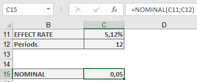

Correlation:
The relationship between nominal and effective interest rates is illustrated in the examples for the EFFECT() function.

ISMA Price and ISMA Yield:
In the semi-annual interest payment example for the PRICE() function, the example includes a reconstruction of the ISMA price using Excel’s built-in function. The yield must be converted using NOMINAL().

This function calculates the modified internal rate of return (MIRR), evaluating negative cash flows (disbursements) and positive cash flows (deposits) at different interest rates.

Syntax:
MIRR(Values; Investment; Reinvestment)

Arguments

• Values (required)
  • A range of cash flows (disbursements and deposits) arranged chronologically.
  • Each value represents the end of a period (e.g., yearly).
  • Must include at least one positive and one negative value.
  • Non-numeric or empty cells are ignored.
• Investment (required)
  • The discount rate applied to negative cash flows (borrowing cost).
• Reinvestment (required)
  • The interest rate applied to positive cash flows (reinvestment yield).

Background

The MIRR method improves upon the standard IRR() by:

1. Separate rates for financing (negative flows) and reinvestment (positive flows).
2. Eliminating multiple IRR issues that arise with irregular cash flows.
3. Providing a realistic reinvestment assumption (unlike IRR, which assumes reinvestment at the IRR itself).

Advantages:

✔ Clear reinvestment rate – Reflects realistic earnings on deposits.
✔ No time horizon limitation – Unlike NPV, which requires a fixed rate.

Disadvantages:

✖ Fixed rates – Assumes constant borrowing and reinvestment rates.

Example

An investor buys a 5-year government bond with:

• Annual coupon rate: 4.25%
• Reinvestment rate: 2% (due to market conditions)

IRR vs. MIRR:

Metric	Calculation	Result
IRR()	Standard return	4.25%
MIRR()	Adjusted for reinvestment	4.08%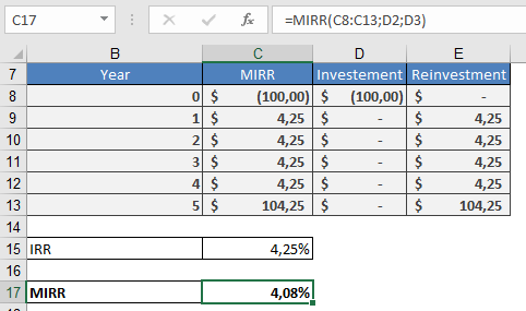

Interpretation:

• Initial investment: $100
• Future value (FV):
  • Coupons reinvested at 2% → $122.12 after 5 years.
• MIRR (4.08%) reflects the true annualized return after accounting for lower reinvestment yields.

Key Takeaway

MIRR provides a more realistic measure of profitability by:

• Using separate rates for costs and reinvestment.
• Avoiding the overstated returns of IRR when reinvestment rates differ.

This function calculates the modified duration for fixed-interest securities.

Syntax:
MDURATION(Settlemen; Maturity; Nominal_Interest; Yield; Frequency; Basis)

Arguments:

• Settlement (required) – The date when ownership of the security is transferred.
• Maturity (required) – The date when the loan (represented by the security) is repaid.
• Nominal_Interest (required) – The annual coupon rate (agreed interest rate) of the security.
• Yield (required) – The market interest rate on the settlement date, used to discount future cash flows in the duration calculation.
• Frequency (required) – The number of interest payments per year. Valid options:
  • 1 = Annual
  • 2 = Semiannual
  • 4 = Quarterly
• Basis (optional) – The day-count convention. If omitted, Excel defaults to Basis = 0.

Notes:

• Date arguments are truncated to integers (no time component).
• Frequency and Basis must be integers (decimal places are truncated).
• Errors:
  • #VALUE! – Invalid dates or non-numeric inputs where required.
  • #NUM! – Invalid numbers for non-date arguments.

Background:
Modified duration measures a bond’s price sensitivity to interest rate changes, crucial for risk management. Unlike stocks, fixed-income securities see reduced price volatility as maturity nears because redemption value is fixed.

Mathematically:

• Duration = Macaulay Duration (see DURATION()).
• MDURATION() returns the scaling factor for estimating relative price change due to interest rate shifts (unsigned).
• For multiple annual payments, the yield is distributed evenly across periods.

Example:
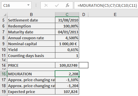
A 4.5% federal bond (issued 2003) had:

• Yield (Aug 31, 2010): 0.61%
• Maturity: Jan 4, 2030
• Price: $109.027

Scenario:

• If yield rises +0.5% (to 1.11%), the price drops to $107.800 (–1.13%).

Using MDURATION():

• Modified Duration = 2.208
• Estimated price change = 2.208 × 0.5% ≈ 1.1% decline
• New price ≈ $107.824 (vs. actual $107.800)

Conclusion:
Modified duration helps investors quickly assess risk without complex recalculations.

Calculates the simple interest accrued for a specific period within a year, based on a fixed annual interest rate. Unlike standard compound interest functions, ISPMT() assumes no intra-period compounding.

Syntax

ISPMT(Rate; Per; Nper; Pv)

Arguments

Argument	Description
Rate	Annual interest rate (e.g., 6%).
Per	Period number (zero-based) or days elapsed (if Nper = 360).
Nper	Total periods in a year (e.g., 12 for months, 360 for days).
Pv	Principal amount (use negative for cash outflow, e.g., -100).

Key Features

• Simple Interest Only: Interest is linear (no compounding).
• Formula:

• Use Case: Legacy systems (e.g., Lotus 1-2-3 compatibility) or scenarios where compounding is irrelevant (e.g., short-term loans).

Examples

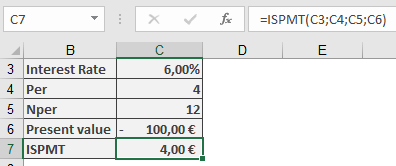
1. Savings Account (Monthly Periods)
   • Deposit: $100 on April 30 (Month 4 of 12).
   • Annual Rate: 6%.
   • Interest for Remaining Year:

=ISPMT(6%, 4, 12, -100) → **$4.00** 

1. Daily Interest Calculation
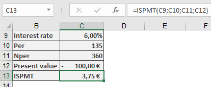
   • Deposit: $100 on May 5 (Day 135 of 360).
   • Interest for Remaining Year:

=ISPMT(6%, 135, 360, -100) → **$3.75** 

Comparison to IPMT()

Feature	ISPMT()	IPMT()
Interest Type	Simple (linear)	Compound (annuity repayment)
Usage	Legacy compatibility	Modern loan/deposit analysis
Periods	Zero-based counting	One-based counting

Limitations

• No Compounding: Not suitable for investments/loans with intra-period compounding.
• Negative Periods: Returns erroneous values if Per ≥ Nper.

Calculates the Internal Rate of Return (IRR)—the discount rate that makes the Net Present Value (NPV) of a series of cash flows equal to zero.

Syntax

IRR(Values; [Guess])

Arguments

Argument	Description
Values (required)	A range/array of cash flows (negative = outflows, positive = inflows). Must include at least one negative and one positive value.
Guess (optional)	Initial estimate for IRR (default: 10%). Helps avoid calculation errors in complex cash flows.

Key Features

• Purpose: Evaluates profitability of investments/projects.
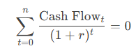
• Formula: Solves for rr in:

• Limitations:
  • May return multiple solutions for irregular cash flows.
  • Fails if cash flows are all positive/negative (#NUM! error).

Examples

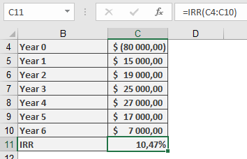
1. Machine Investment
   • Initial Cost: -$80,000 (Year 0).
   • Annual Surpluses:

Year	Cash Flow
1	$15,000
2	$19,000
…	…
6	$7,000

1. • Calculation:

=IRR(B2:B8) → **10.47%** 

1. • Interpretation: IRR (10.47%) > Hurdle Rate (10%) → Viable investment.
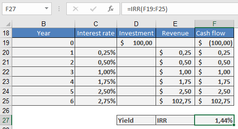
2. Federal Savings Bond
   • Cash Flows: Fixed annual interest payments.
   • Result:

=IRR(C2:C8) → **1.44%** 

1. • Note: Matches the German Federal Bank’s published yield.

Practical Tips

• Guess Argument: Use for complex cash flows (e.g., IRR(Values, 5%)).
• Validation: Cross-check with NPV(IRR(Values), Values) ≈ 0.
• Alternatives: Use XIRR() for irregularly timed cash flows.

Common Errors

Error	Cause	Fix
#NUM!	No convergence after 20 iterations.	Adjust Guess or verify cash flow signs.
#VALUE!	Non-numeric data in Values.	Ensure all inputs are numbers.

 

Its calculates the interest portion of a fixed periodic payment (annuity) for a loan or investment under the annuity repayment method.

Syntax

IPMT(Rate; Per; Nper; Pv; [Fv]; [Type])

Arguments

Argument	Description
Rate (required)	Periodic interest rate (e.g., 5.5%/12 for monthly payments).
Per (required)	Specific period number (e.g., 18 for the 18th payment).
Nper (required)	Total number of payment periods (e.g., 30*12 for a 30-year loan).
Pv (required)	Present value (loan principal).
Fv (optional)	Future value (residual value after Nper). Default: 0.
Type (optional)	0 = end of period (default), 1 = start of period.

Key Features

• Annuity Repayment: Payments combine interest (decreasing over time) and principal (increasing over time).
• Formula:

Interest in Period=Remaining Principal×RateInterest in Period=Remaining Principal×Rate

• Sign Convention:
  • Negative result: Cash outflow (e.g., loan interest paid).
  • Positive result: Cash inflow (e.g., interest earned on investments).

Example

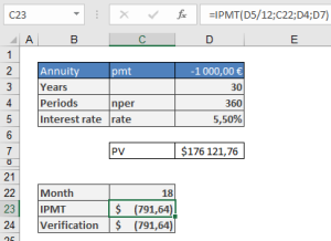
Loan Repayment Calculation

• Loan Amount (Pv): $176,121.76
• Annual Rate: 5.5% → Monthly Rate: 5.5%/12
• Term: 30 years → 360 months (Nper = 30*12)
• 18th Month Interest:

=IPMT(5.5%/12, 18, 360, 176121.76) → **-$791.64** 

(Interest paid in the 18th month)

Practical Notes

1. Rounding Errors:
   • Banks round to 2 decimal places. Use ROUND(IPMT(…), 2) for accuracy.
2. Full Payment Plan:
   • Combine with PPMT() (principal portion) to verify total payment:

=IPMT(Rate, Per, Nper, Pv) + PPMT(Rate, Per, Nper, Pv) = PMT(Rate, Nper, Pv) 

1. Type Matters:
   • For leases/advance payments, set Type=1.

Comparison to Related Functions

Function	Purpose
PMT()	Total periodic payment (interest + principal).
PPMT()	Principal portion of payment.
CUMIPMT()	Cumulative interest over multiple periods.

Its calculates the equivalent annual interest rate (in arrears) for a discounted security (e.g., zero-coupon bond) with intra-year maturity.

Syntax

INTRATE(Settlement; Maturity; Investment; Repayment; [Basis])

Arguments

Argument	Description
Settlement (required)	Purchase date of the security (time truncated).
Maturity (required)	Maturity/redemption date (time truncated).
Investment (required)	Purchase price (must be > 0).
Repayment (required)	Redemption value at maturity (must be > 0).
Basis (optional)	Day-count convention (see Table 15-2). Default: 0 (US 30/360).

Error Handling

• #VALUE! → Invalid dates or non-numeric inputs.
• #NUMBER! → If:
  • Investment ≤ 0 or Repayment ≤ 0.
  • Basis < 0 or > 4.
  • Settlement ≥ Maturity.

Background

• Anticipative vs. Arrears Yield:
  • Anticipative (DISC): Interest deducted upfront (e.g., T-bills).
  • Arrears (INTRATE): Interest paid at maturity (converted to annual equivalent).
• Formula:

• Comparison: Use to contrast with fixed-income securities paying periodic interest.

Example

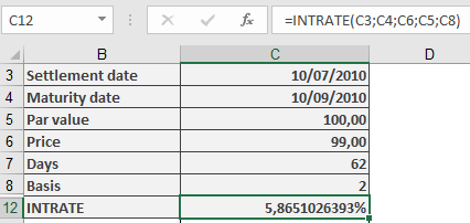
Treasury Bill (T-Bill) Calculation

• Purchase Date: 10, 07, 2010
• Maturity: 10, 09, 2010
• Purchase Price (Investment): $99
• BASIS: 2
• Par Value: 100

=INTRATE(« 10/09/2010 », « 10/09/2010 », 99, 100, 2) 

Result: 5.87% annual yield.

Key Notes

1. No Compounding: Simple interest only.
2. Inverse of DISC(): Converts discount rate to equivalent annual yield.
3. Use Case: Compare short-term securities (e.g., commercial paper, T-bills).

Calculates the future value of an initial investment (Principal) after applying a series of variable compound interest rates over successive periods.

Syntax

FVSCHEDULE(Principal; Schedule)

Arguments

• Principal (required)
  The initial investment amount. Must be a numeric value.
• Schedule (required)
  An array of interest rates for each period (e.g., {0.02, 0.03, 0.025}).
  • Can be a range reference (e.g., C2:C7) or a hardcoded array (e.g., {0.01, 0.02}).
  • Non-numeric values → #VALUE! error.
  • Empty cells → Treated as 0% interest for that period.

Key Features

• Variable Rates: Each period’s interest rate can differ (unlike FV(), which uses a fixed rate).
• Compound Interest: Interest earned in each period is reinvested.

Example

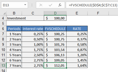
German Federal Savings Bonds (Type B)
Scenario: A €100 bond with annual interest rates as follows:

Year	Interest Rate
2010–2011	0.25%
2011–2012	0.50%
2012–2013	1.00%
2013–2014	1.75%
2014–2015	2.50%
2015–2016	2.75%
2016–2017	2.75%

Calculation:

=FVSCHEDULE(100; {0.0025; 0.005; 0.01; 0.0175; 0.025; 0.0275; 0.0275}) 

Result: €112.23 (future value after 7 years).

Practical Use Cases

1. Savings Bonds: Calculate maturity value with fluctuating annual rates.
2. Variable-Rate Investments: Project returns for funds with non-fixed yields.
3. Loan Analysis: Estimate future debt under changing interest terms.

Comparison to FV()

Feature	FVSCHEDULE()	FV()
Interest Rates	Variable per period	Fixed for all periods
Compounding	Automatic	Requires manual adjustment
Use Case	Bonds, variable-rate accounts	Fixed annuities, loans

Notes

• Negative Rates: Supported (e.g., -0.01 for a 1% loss in a period).
• Zero Rates: Omit or use 0 (no growth for that period).
• Equivalent Fixed Rate: Use RATE() to find the constant rate yielding the same result.

Calculates the future value of an investment or loan based on periodic, constant payments and a constant interest rate.

Syntax

FV(Rate; Nper; Pmt; [Pv]; [Type])

Arguments

• Rate (required)
  The interest rate per period (e.g., 4.5% annual → 4.5%/12 for monthly).
• Nper (required)
  The total number of payment periods (e.g., 15 years × 12 months = 180).
• Pmt (optional)
  The regular payment per period (annuity). Use 0 if omitted.
  • Sign Convention:
    • Negative (-): Cash outflow (e.g., deposits, loan payments).
    • Positive (+): Cash inflow (e.g., withdrawals, dividends).
• Pv (optional)
  The present value (initial lump sum). Defaults to 0.
• Type (optional)
  • 0 (default): Payments at end of period (ordinary annuity).
  • 1: Payments at start of period (annuity due).

Error Handling

• Ensure Rate, Nper, Pmt, and Pv are numeric to avoid #VALUE!.
• Nper must be ≥ 1.

Background

FV() solves the time value of money equation:

Examples

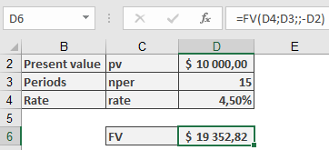
1. Compound Interest (Lump Sum)
   • Scenario: $10,000 invested at 4.5% annual interest for 15 years.
   • Formula:

=FV(4.5%, 15, , -10000) → **$19,352.82**

1. • Note: Pv is negative (cash outflow).
2. Loan Repayment (Residual Debt)
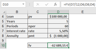
   • Scenario: $100,000 loan at 5.5% annual interest, $1,000 monthly payments for 5 years.
   • Formula:

=FV(5.5%/12, 5*12, -1000, 100000) → **$62,689.55** (remaining balance) 

Key Notes

• Sign Convention: Payments out are negative; inflows are positive.
• Compounding: For loans, interest is typically nominal (e.g., monthly rate = annual rate/12).
• Annuity Types: Type=1 for payments at period start (e.g., leases).

Calculates the effective annual interest rate (compounded) from a nominal annual rate, accounting for intra-year compounding periods.

Syntax

EFFECT(Nominal_Interest; Periods)

Arguments

• Nominal_Interest (required)
  The stated annual nominal interest rate (e.g., 0.05 for 5%). Must be > 0.
• Periods (required)
  The number of compounding periods per year (e.g., 12 for monthly). Must be ≥ 1 (decimal places truncated).

Error Handling

• #VALUE! if non-numeric inputs are provided.
• #NUMBER! if:
  • Nominal_Interest ≤ 0.
  • Periods < 1.

Background

• Nominal vs. Effective Rates:
  • Nominal rates ignore compounding (e.g., 5% annual, paid monthly = 5%/12 per period).
  • Effective rates reflect actual annual yield after compounding (e.g., 5% nominal → ~5.12% effective for monthly compounding).
• Formula:

Examples

1. Savings Account
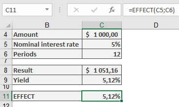
   • Scenario: $1,000 deposited at 5% nominal interest, compounded monthly.
   • Calculation:

=EFFECT(5%, 12)  → Returns **5.12%**

1. • Verification:
     • Monthly interest: 5%/12 = 0.4167%.
     • Year-end balance: =FV(5%/12, 12, , -1000) = $1,051.16.
     • Effective yield: (1051.16 / 1000) – 1 = 5.12%.

1. Mortgage Loan
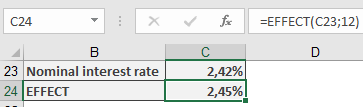
   • Scenario: Bank offers 2.42% nominal rate, compounded monthly.
   • Calculation:

=EFFECT(2.42%, 12)  → Returns **2.45%** (matches advertised effective rate). 

1. • Note: Banks may use alternative methods; exact matches may be coincidental.

Key Points

• Comparison Tool: Use to compare loans/investments with different compounding frequencies.
• Limitations: Assumes reinvestment at the same rate; does not account for fees or irregular payments.