Votre panier est actuellement vide !
Catégorie : Excel function
How to use the COUPDAYSNC() Function in Excel
Calculates the number of days from the settlement date to the next coupon payment date for a fixed-income security.
Syntax
COUPDAYSNC(Settlement; Maturity; Frequency; Basis)
Arguments
Argument Required Description Valid Values Settlement Yes Date ownership transfers Valid date (time truncated) Maturity Yes Bond repayment date Must be after Settlement Frequency Yes Coupon payments per year 1, 2, or 4 Basis No Day-count method 0-4 (default=0) Day-Count Basis Methods
Basis Method Key Characteristic 0 30/360 (NASD) Standard financial convention 1 Actual/Actual Exact day count 2 Actual/360 Money market convention 3 Actual/365 British convention 4 30/360 (European) Eurobond convention Key Features
- Primary Use:
- Determines days until next coupon payment
- Essential for calculating:
- Accrued interest allocations
- Present value of future cash flows
- Error Handling:
- #VALUE!: Invalid date format
- #NUM!:
- Invalid Frequency/Basis
- Settlement ≥ Maturity
- Calculation Method:
- Automatically identifies next coupon date
- Applies specified day-count convention
EXAMPLE
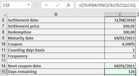
Common Implementation Errors
- Using maturity date as settlement
- Incorrect Basis for security type
- Forgetting to truncate time values
- Primary Use:
How to use the COUPDAYS() Function in Excel
Calculates the total number of days in the coupon period that contains the settlement date for a fixed-income security.
Syntax
COUPDAYS(Settlement; Maturity; Frequency; Basis)
Arguments
Argument Required Description Valid Values Settlement Yes Date of ownership transfer Valid Excel date Maturity Yes Bond repayment date Must be after Settlement Frequency Yes Interest payments per year 1 (annual), 2 (semi-annual), 4 (quarterly) Basis No Day-count convention 0-4 (default=0) Day-Count Basis Methods (Table 1)
Basis Method Description 0 30/360 (NASD) 30-day months, 360-day year 1 Actual/Actual Exact calendar days 2 Actual/360 Actual days/360-day year 3 Actual/365 Actual days/365-day year 4 30/360 (European) European 30-day convention Requirements & Error Handling
- Dates must be valid (time components are ignored)
- Frequency and Basis are converted to integers
- Returns #VALUE! for:
- Invalid date formats
- Text instead of dates
- Returns #NUM! for:
- Invalid Frequency (not 1, 2, or 4)
- Invalid Basis (not 0-4)
- Settlement date later than Maturity date
Background
- Determines the length of the current coupon period
- Essential for calculating:
- Accrued interest
- Day-count fractions for yield calculations
- Different day-count methods produce slightly different results
- Used in conjunction with other coupon functions (COUPDAYBS, COUPDAYSNC)
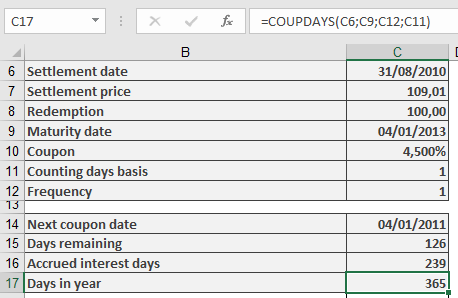
Example Applications
Key Notes
- For US corporate bonds: Typically Basis=0 (30/360)
- For government bonds: Typically Basis=1 (Actual/Actual)
- Always verify Settlement date precedes Maturity date
- Combine with COUPNUM() and COUPPCD() for complete coupon analysis
- Critical for accurate dirty price calculations in bond trading
How to use the COUPDAYBS() Function in Excel
Calculates the number of days between the last coupon payment date and the settlement date for a fixed-income security with regular interest payments.
Syntax
COUPDAYBS(Settlement; Maturity; Frequency; Basis)
Arguments
Argument Required Description Valid Values Settlement Yes Date of ownership transfer Valid date format Maturity Yes Bond repayment date Must be after Settlement Frequency Yes Interest payments per year 1 (annual), 2 (semi-annual), 4 (quarterly) Basis No Day-count convention (see Table 1) 0-4 (default=0) Day-Count Basis Methods (Table 1)
Basis Method Description 0 30/360 (NASD) 30-day months, 360-day year 1 Actual/Actual Exact calendar days 2 Actual/360 Actual days/360-day year 3 Actual/365 Actual days/365-day year 4 30/360 (European) European 30-day convention Requirements & Error Handling
- Dates must be valid (no time component)
- Frequency and Basis are truncated to integers
- Returns #VALUE! for invalid dates
- Returns #NUM! for:
- Invalid Frequency (≠1,2,4)
- Invalid Basis (≠0-4)
- Settlement date > Maturity date
Background
- Used to calculate accrued interest owed when bonds trade between coupon dates
- Different day-count methods yield slightly different results
- Essential for accurate bond pricing and yield calculations
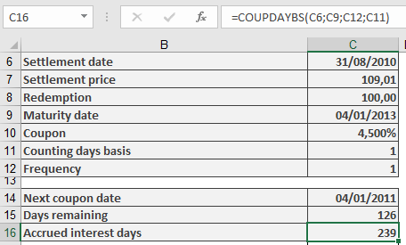
Example Applications
- Accrued Interest Calculation:
Accrued Interest = (Annual Coupon Rate × Face Value) × (COUPDAYBS()/Days in Coupon Period)
- Yield Analysis:
- Used with YIELD() and PRICE() functions
- Helps determine exact holding period returns
Key Notes
- For US corporate bonds: Typically Basis=0 (30/360)
- For government bonds: Typically Basis=1 (Actual/Actual)
- Always verify Settlement < Maturity
- Combine with COUPNCD() and COUPPCD() for complete coupon date analysis
How to use the AMORLINC() function in Excel
This function calculates the linear depreciation of an asset for a specified period, following the French accounting system. Unlike AMORDEGRC() (which uses degressive depreciation), AMORLINC() applies a straight-line method, making it adaptable to other tax jurisdictions with minor adjustments.
Syntax
AMORLINC(Cost; Date; First_Period; Residual_Value; Period; Rate; Basis)
Arguments
Table 1
Argument Description Cost (required) Total purchase cost (including expenses, minus discounts). Must be positive; otherwise, returns #VALUE! or #NUMBER!. Date (required) Asset purchase date (depreciation start date). First_Period (required) End date of the first depreciation period (assigned period 0). Residual_Value (required) Expected remaining value post-depreciation. Must be ≤ Cost and non-negative; otherwise, returns #NUMBER!. Period (required) Depreciation period (integer ≥ 0). Rate (required) Annual depreciation rate (e.g., 10% for 10 years, 20% for 5 years). Basis (optional) Day-count method (see Table 2 below). Default varies by region. Table 2: Day-Count Methods
Basis Method Description 0 30/360 (NASD) 30-day months, 360-day year. Adjusts 31st to 30th. 1 Exact/Exact Actual days per month/year. 2 Exact/360 Actual days/month; year = 360 days. 3 Exact/365 Actual days/month; year = 365 days. 4 30/360 (European) 30-day months; converts 31st to 30th. Key Notes
- First Period (Period 0):
- Depreciation is prorated based on days counted (per Basis).
- Example: Purchase in October → First period covers October–December.
- Residual Value Handling:
- If residual = 0: Depreciation may extend beyond the planned periods to account for partial-year start.
- If residual > 0: Depreciation stops when book value ≤ residual.
- Tax Law Adaptations:
- For German tax law, use Basis = 4 and set:
- Date = First day of the purchase month.
- First_Period = January 1 of the next year.
- Avoid using month-end dates (e.g., February 28) to prevent day-count errors.
- For German tax law, use Basis = 4 and set:
Example
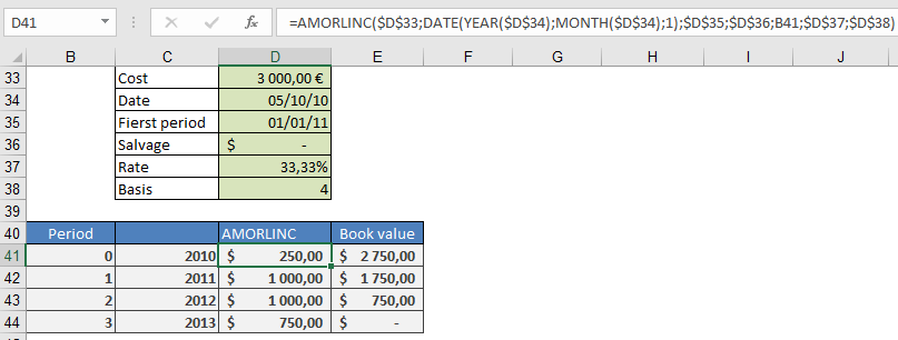
Scenario: Purchase a $3,000 computer on October 5, 2010, with:
- Depreciation rate: 33.333% (3-year lifespan).
- Residual value: $0.
- First period ends: January 1, 2011.
Formula
=AMORLINC(3000, DATE(2010,10,1); « 1/1/2011 »; 0; 0; 33.333%; 4)
Result: $250.00 (depreciation for October–December 2010).
Manual Calculation
- Days in first period:
=DAYS360(DATE(2010,10,1); « 1/1/2011 »; TRUE) → 90 days
- Depreciation:
=3000 × 33.333% × (90/360) → $250.00
Alternative:
=3000 × 33.333% × (3 months / 12) → $250.00
Why Use AMORLINC?
- Simplicity: Straight-line method avoids complex degressive calculations.
- Flexibility: Adaptable to various tax laws with proper Basis selection.
- Accuracy: Handles partial-year depreciation seamlessly.
- First Period (Period 0):
How to use the AMORDEGRC() function in Excel
This function calculates the depreciation amount for an asset in a given period using the French accounting system (degressive depreciation with a switch to linear). The result is rounded to an integer.
Syntax
AMORDEGRC(Cost; Date; First_Period; Residual_Value; Period; Rate; Basis)
Arguments
- Cost (required) – Purchase cost of the asset (including incidental expenses, minus discounts).
- Must be a positive number; otherwise, #VALUE! or #NUMBER! errors occur.
- Date (required) – The purchase date (start of depreciation).
- First_Period (required) – The end date of the first depreciation period (assigned period number 0).
- Residual_Value (required) – Expected remaining value after depreciation.
- Must be less than Cost and non-negative; otherwise, #NUMBER! is returned.
- Period (required) – The time period for which depreciation is calculated (integer ≥ 0).
- Rate (required) – The depreciation rate (initially linear, then degressive).
- Basis (optional) – Day-count method (see Table 1 below).
Table 1: Day-Count Methods
Basis Method Description 0 30/360 (NASD) Months = 30 days; years = 360 days. Adjusts 31st to 30th. 1 Exact/Exact Actual days per month/year. 2 Exact/360 Actual days/month; year = 360 days. 3 Exact/365 Actual days/month; year = 365 days. 4 30/360 (European) Months = 30 days; years = 360 days. Converts 31st to 30th. Background
- Depreciation reflects the asset’s value loss (not physical wear).
- The Rate is first treated as linear (e.g., 10% = 10-year lifespan).
- Degressive weighting is applied based on the rate:
- Factor 1.5 if Rate > 25% (3–4 years).
- Factor 2 if 16.66% ≤ Rate ≤ 25% (5–6 years).
- Factor 2.5 if Rate < 16.67% (>6 years).
- Residual value handling:
- If residual = 0, the last two periods split the remaining value.
- If residual > 0, depreciation stops when book value ≤ residual.
Example
An asset is purchased on June 6, 2010, for $1,000, with:
- Depreciation rate: 10%
- Residual value: $142
- First period ends: December 31, 2010
Formula
=AMORDEGRC(1000; « 6/6/2010 »; « 12/31/2010 »; 142; 0; 10%; 4)
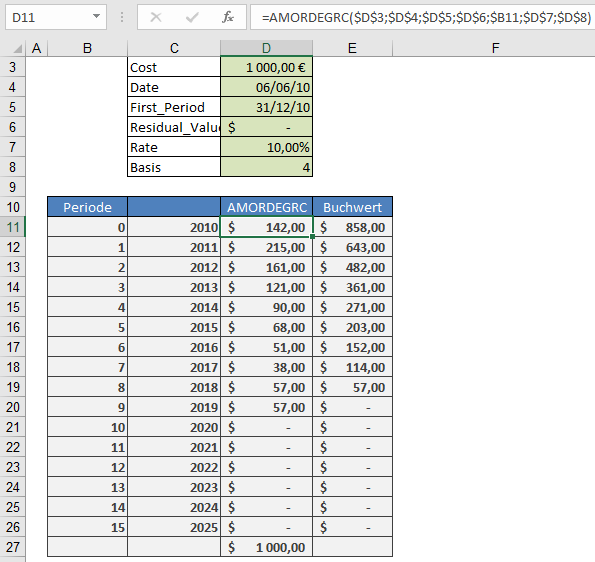
Manual Calculation
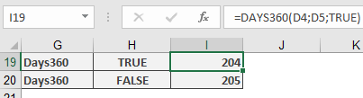
- Days in first period:
=DAYS360(« 6/6/2010 »; « 12/31/2010 »; TRUE) → 204 days
- Depreciation:
=ROUND(1000 × 10% × 2.5 × (204/360); 0) → $142 (matches AMORDEGRC).
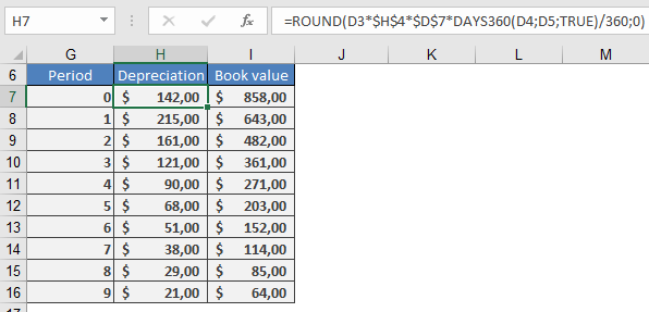
Subsequent Periods
- Multiply the previous book value by 10% × 2.5.
- Cost (required) – Purchase cost of the asset (including incidental expenses, minus discounts).
How to use the ACCRINTM() function in Excel
The ACCRINTM() function calculates the accrued interest of a debt instrument (such as a bond or loan) that has a single interest payment at maturity. This is a simplified version of ACCRINT(), designed for securities with one annual interest period.
Syntax
ACCRINTM(Issue; Settlement; Nominal_Interest; Par_Value; Basis)
Arguments
- Issue (required) – The issuance date of the security.
- Settlement (required) – The date when ownership of the security changes.
- Nominal_Interest (required) – The annual interest rate of the security.
- Par_Value (optional) – The nominal value of the security. If omitted, Excel defaults to 1000 (contrary to older Excel Help documentation).
- Basis (optional) – Day-count convention.
Notes
- Dates must be entered without time values (decimals are truncated).
- Basis must be an integer (decimals are truncated).
- Errors:
- #VALUE! – Invalid dates or non-numeric entries.
- #NUMBER! – Invalid numeric inputs.
Background
- This function is specifically for single-payment securities (e.g., zero-coupon bonds or loans due in full at maturity).
- Unlike ACCRINT(), which handles periodic interest payments, ACCRINTM() assumes one annual interest period.
- The calculation method aligns with ACCRINT(), but with a simplified structure.
Examples
- Debt Due in Full
A $1,000 debt issued on June 1, 2010, with:
- 4% annual interest
- Ownership change on August 9, 2010
Formula:
=ACCRINTM(C2, C3, 4%, 1000, 4)- C2 = Issue date (June 1, 2010)
- C3 = Settlement date (August 9, 2010)
Result:

Calculates the accrued interest from issuance to settlement.- German Federal Government Bond (WKN 113517)
- Issued: October 25, 2000
- Nominal Interest: 5.5% (annual)
- Maturity: January 4, 2031
- Purchase Date: August 30, 2010
- Market Price: €143.27
Formula:
=ACCRINTM(C24, C25, 5.5%, 100, 4)- C24 = Last interest payment date (January 4, 2010)
- C25 = Settlement date (August 30, 2010)
Result:
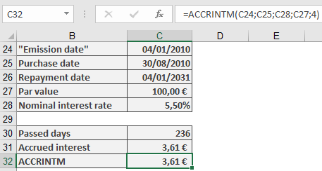
- Accrued Interest: €3.61 per bond
- Total Payment: €143.27 (price) + €3.61 (interest) = €146.88
How to use the ACCRINT() Function in Excel
The calculates accrued interest for:
- Debt instruments due in full intra-annually
- Fixed-interest securities with periodic payments
Syntax
ACCRINT(Issue; First_Interest_Date; Settlement; Nominal_Interest; Par_Value; Frequency; Basis; Calculation_Method)
Arguments
Argument Required? Description Notes Issue Yes Date of issuance Must be valid date First_Interest_Date Yes First coupon date For intra-annual debt = due date Settlement Yes Ownership transfer date Must be ≥ Issue date Nominal_Interest Yes Annual coupon rate Decimal format (4% = 0.04) Par_Value No Face value Default = 1000 Frequency Yes Payments per year 1, 2, or 4 Basis No Day-count method 0-4 (Default=0) Calculation_Method No Interest calculation TRUE (full duration) or FALSE (since last payment) Day-Count Methods (Basis)
Basis Method Description 0 30/360 (NASD) Standard 30-day months 1 Actual/Actual Exact days 2 Actual/360 Bankers’ year 3 Actual/365 Exact days/365 4 30/360 (European) Eurobond standard Key Features
- Accrued Interest Calculation:
- For multiple annual payments: (Nominal_Interest/Frequency) × (Days held/Days in period)
- Uses specified day-count method (Basis)
- Error Handling:
- #VALUE! – Invalid dates
- #NUMBER! – Negative values or invalid numbers
- Special Cases:
- First period (Period 0) is prorated
- When Calculation_Method=FALSE, only calculates since last payment
Practical Example
Scenario: $1,000 debt issued June 1, 2010, due December 1, 2010 (4% annual rate), sold August 9, 2010.
Solution:
- Accrued Interest (68 days held):
=ACCRINT(« 6/1/2010″, »12/1/2010″, »8/9/2010 »,4%,1000,1,4)
Returns: $7.56
Manual verification:
1000 × 4% × (68/360) = $7.56

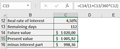
- Present Value Calculation (112 days remaining):
- Future value: $1,020 (principal + 6mo interest)
- Discounted at 4.5%:
$1,020 / (1 + 0.045 × (112/360)) = $1,005.92
Pro Tips
- For German bonds, use Basis=4 (30/360 European)
- Combine with PRICEMAT() for full valuation:
=(PRICEMAT(…)×10) + ACCRINT(…)
- Verify calculations using:
- DAYS360() for day counts
- COUPDAYBS() for days since last coupon
Common Use Cases
- Bond transactions between coupon dates
- Loan transfers with accrued interest
- Financial reporting for interest receivables
How to use the Z.TEST() function in Excel
This function returns the one-tailed probability value for a Gauss test (normal distribution). For a given expected value of a random variable (μ0), the Z.TEST() function returns the probability that the sample mean would be greater than the average of observations in the data set (array)—that is, the observed sample mean.
Syntax
Z.TEST(array ; μ0 ; sigma)
Arguments
- array (required) – The array or range of data against which to test μ0.
- μ0 (required) – The value to test.
- sigma (optional) – The known standard deviation of the population. If omitted, the sample standard deviation is used.
Notes
- If array is empty, Z.TEST() returns the #N/A error.
- The calculation differs depending on whether sigma is provided:
When sigma is specified:

When sigma is omitted:

Where:
-
- x̄ = sample mean (AVERAGE(array))
- s = sample standard deviation (STDEV.S(array))
- n = number of observations (COUNT(array))
- Φ = standard normal cumulative distribution function
- Z.TEST() indicates the probability that the sample mean is greater than the observed mean (AVERAGE(array)) when the expected value is μ0.
- Due to the symmetry of the normal distribution, if AVERAGE(array) < μ0, Z.TEST() returns a value greater than 0.5.
- For a two-tailed probability test, use:
=2×MIN(Z.TEST(array,μ0,sigma),1−Z.TEST(array,μ0,sigma))=2×MIN(Z.TEST(array,μ0,sigma),1−Z.TEST(array,μ0,sigma))
Background
The Gaussian test (named after mathematician Carl Friedrich Gauss) is a statistical test based on the standard normal distribution. It examines the significance of a value from a normally distributed population where the expected value (μ0) and standard deviation (sigma) must be known.
Example
Calculate Z.TEST() using the following parameters:
- Data = The range of values to test against μ0
- μ0 = 4 (first test value)
- μ0 = 6 (second test value)
Results (as shown in Figure below):
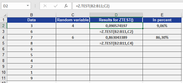
- For μ0 = 4, the one-tailed probability is 0.09057 (9.06%).
- For μ0 = 6, the one-tailed probability is 0.86304 (86.30%).
How to use the WEIBULL.DIST() function in Excel
This function returns values of a Weibull-distributed random variable. It is typically used in reliability analysis, such as calculating the mean time to failure of a device.
Syntax. WEIBULL.DIST(x; alpha; beta; cumulative)
Arguments- x (required): The value at which the function is to be evaluated.
- alpha (required): A shape parameter of the distribution.
- beta (required): A scale parameter of the distribution.
- cumulative (required): A logical value that specifies the form of the function:
— If TRUE, WEIBULL.DIST() returns the cumulative distribution function (CDF)—i.e., the probability that the event occurs between 0 and x.
— If FALSE, the function returns the probability density function (PDF)—i.e., the value of the density function at x.
Background
The Weibull distribution is a statistical distribution widely used to model life expectancy and failure rates, especially for brittle materials or electronic components.
Named after Waloddi Weibull (1887–1979), this distribution is a cornerstone in reliability engineering and is commonly visualized using a Weibull plot—often called a Weibull net—which represents life cycles and failure probabilities of mechanical or electronic parts. It is frequently used in the automotive industry.
In essence, the Weibull distribution can represent various types of data depending on its parameters. It is flexible, mathematically simple to calculate, and can model:
- Early-life failures (infant mortality),
- Random failures (constant failure rate),
- Wear-out failures (increasing failure rate).
Key properties:
- The distribution function (CDF) indicates the probability that a random variable y is less than or equal to x.
- The density function (PDF) is the derivative of the distribution function with respect to x, representing the failure rate at a specific point in time.
To calculate:
- The density function, set cumulative = FALSE.
- The distribution function, set cumulative = TRUE.
Formulas
- Cumulative Distribution Function (CDF):

- Density Function (PDF):
The first derivative of the distribution function with respect to x.
Note: If α = 1, WEIBULL.DIST() becomes an exponential distribution.
- Failure rate behavior depends on α:
- If α < 1, failure rate decreases over time (early failures).
- If α = 1, failure rate is constant (random failures).
- If α > 1, failure rate increases over time (wear-out failures).
Example
Let’s compute values using WEIBULL.DIST() with the following parameters:
- x = 105 (value to evaluate)
- alpha = 20
- beta = 100
- cumulative = TRUE / FALSE
As shown in Figure below, the function returns:
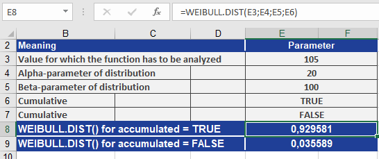
- For cumulative = TRUE: 0.929581 (CDF – cumulative probability up to 105)
- For cumulative = FALSE: 0.035589 (PDF – probability density at 105)
How to use the VARPA() function in Excel
This function calculates the variance based on the entire population. Unlike VAR.P(), VARPA() includes numbers, text, and logical values (TRUE and FALSE) in its calculation.
Syntax. VARPA(value1; value2; …)
Arguments- value1 (required) and
- value2 (optional)
You can enter at least one and up to 255 values, representing the population data set.
Background
Since variance has already been explained in the description of VAR.S(), this section focuses on the example.
VARPA() uses the same formula as VAR.P():
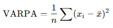
Where:
- xˉ is the population mean, calculated by AVERAGE(value1; value2; …)
- n is the number of values in the population
Like VARA(), the VARPA() function treats text and logical values as follows:
- Text entries and the logical value FALSE are treated as 0
- TRUE is treated as 1
Example
The same scenario used for the VARA() function also applies here. The software company experienced several website issues over the observed period:
- In May 2007 and August 2007, the website was unavailable due to hosting problems. These months are marked with the text « hostingproblems ».
- In March 2008, the product section was updated, preventing external access. This month is marked with the logical value FALSE.
As shown in Figure below, the result of the VARPA() function differs from that of VAR.P() because VARPA() includes text and logical values in the calculation.
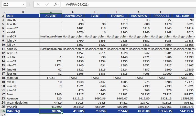
In this case, the text and the logical value FALSE are treated as 0, which affects the variance.
Looking at the DOWNLOAD section, the result can be summarized as follows:
The average squared deviation from the arithmetic mean—based on the population and including text and logical values—is 419,085 for the DOWNLOAD area.