Catégorie : Excel function

Its calculates the price per $100 face value of a discounted security that uses anticipative interest (discount interest applied upfront).

Syntax

PRICEDISC(Settlement; Maturity; Disc; Repayment; [Basis])

Arguments

Argument	Requirement	Description	Validation
Settlement	Required	Trade settlement date	Valid date ≤ Maturity
Maturity	Required	Security maturity date	Valid date ≥ Settlement
Disc	Required	Annual discount rate	> 0
Repayment	Required	Redemption value per $100 face value	> 0
[Basis]	Optional	Day count convention (0-4)	Default=0

Error Conditions

• #VALUE!: Invalid dates or non-numeric inputs
• #NUM!: Negative rates or invalid Basis

Key Features

1. Uses anticipative interest model:
   • Interest deducted upfront (disagio)
   • Contrasts with standard arrears interest
2. Common applications:
   • Treasury bills
   • Commercial paper
   • Bankers’ acceptances

Calculation Method

Price = Repayment × (1 – Disc × DSM/DIM)

Where:

• DSM = Days from settlement to maturity
• DIM = Days in year per Basis convention

Examples

1. German Treasury Bond

Terms:

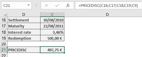
• Face value: €500
• Settlement: 30-Aug-2010
• Maturity: 22-Aug-2011
• Discount: 0.46%
• Basis: 1 (actual/actual)

Calculation:

=PRICEDISC(« 30/8/2010″, »22/8/2011 »,0.46%,500,1)

Result: €497.75

Equivalent Yield Calculation:

=RECEIVED(« 30/8/2010″, »22/8/2011 »,497.75,500,1)

Returns: 0.46% (matches Bundesbank published rate)

Important Notes

1. Day Count Conventions:
   • Basis 0: US (NASD) 30/360
   • Basis 1: Actual/actual
   • Basis 2: Actual/360
   • Basis 3: Actual/365
   • Basis 4: European 30/360
2. Financial Context:
   • Primarily for short-term instruments (<1 year)
   • Low-yield environments may show minimal price differences
   • For precise institutional calculations, verify day count rules
3. Complementary Functions:
   • YIELDDISC(): Calculates equivalent yield
   • RECEIVED(): Determines maturity amount

This function calculates the price of a fixed-income security (loan), meaning the purchase price excluding any accrued interest.

Syntax.
PRICE(Settlement; Maturity; Rate; Yield; Redemption; Frequency; Basis)

Arguments

• Settlement (required): The date on which the ownership of the security changes.
• Maturity (required): The date on which the loan represented by the security is repaid.
• Rate (required): The agreed-upon annual interest rate for borrowing the money.
• Yield (required): The market interest rate on the settlement date, used to discount all future payments during the calculation of the term.
• Redemption (required): The percentage of the par value of the security (assuming a nominal value of 100 monetary units) repaid at maturity.
• Frequency (required): Specifies the number of coupon payments per year. Accepted values:
  • 1 = annual,
  • 2 = semiannual,
  • 4 = quarterly.
• Basis (optional): Defines the day count basis according to Table 15-2 referenced earlier. If omitted, Excel uses Basis = 0.

Requirements for PRICE() Arguments:

• Dates must not contain time values; decimals are truncated.
• Frequency and Basis are truncated to integers.
• If a date argument is invalid, the function returns the #NUM! error.
• Rate and Yield must be non-negative. Redemption must be positive. Otherwise, PRICE() returns the #VALUE! error.
• If Frequency is not 1, 2, or 4, or if Basis is not between 0 and 4, or if the Settlement date is later than Maturity, the function returns #NUM!.

Background.
To apply the financial principle of equivalence:
Payment by creditor = Payment by debtor

At the beginning of the transaction, the price of a fixed-income security (loan) plus accrued interest equals the present value of the debtor’s future payments stipulated by the security. The price represents a percentage of the security’s par value, assuming a par value of 100 monetary units.

When the purchase date coincides with the interest payment date for a security with annual interest payments, calculating the present value is straightforward—only the full year needs consideration. However, when ownership changes between coupon dates or when multiple coupon payments occur per year, the calculation becomes more complex. Several financial methods address this, with the most notable being Moosmüller, Braess/Fangmeyer, and ISMA (International Securities Market Association, formerly Association of International Bond Dealers, AIBD).

The ISMA method yields the same result as PRICE() for annual payments and can be adapted for semiannual and quarterly payments using the PRICE() function.

Excel Approach:
In Excel and related functions, cash value creation (discounting future payments) is performed as follows: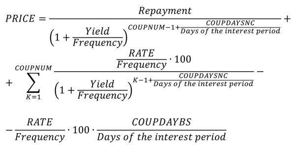

• COUPNUM: Number of coupon payments remaining after settlement.
• COUPDAYSNC: Number of days until the next coupon payment.
• COUPDAYBS: Number of days since the last coupon payment.

When Frequency = 1, this formula aligns with the ISMA method. For Frequency values of 2 or 4, Excel assumes an even distribution of Yield over the year’s periods. In contrast, the ISMA method uses a more complex period apportionment based on the relationship between nominal and effective interest, as explained in the EFFECT() and NOMINAL() function descriptions.

Thus, for multiple coupon payments per year, you can use PRICE() to calculate the ISMA price—but you must first convert the effective yield to a nominal yield using NOMINAL().

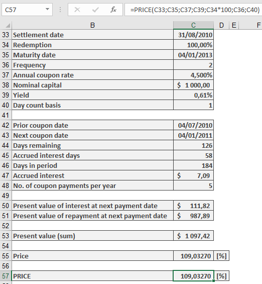
Example.

Its calculates the principal payment portion of a fixed payment (annuity) for a specific period of an investment or loan with constant payments and interest rate.

Syntax

PPMT(Rate; Per; Nper; Pv; [Fv]; [Type])

Arguments

Argument	Requirement	Description
Rate	Required	Interest rate per period
Per	Required	Period number for which to calculate principal payment (1 to Nper)
Nper	Required	Total number of payment periods
Pv	Required	Present value (total loan amount)
[Fv]	Optional	Future value/remaining balance after last payment (default=0)
[Type]	Optional	Payment timing: 0=end of period (default), 1=beginning

Background

In annuity-based loan repayment:

• Each payment contains:
  • Principal portion (increases over time)
  • Interest portion (decreases as loan balance reduces)
• First period principal = Payment – (Loan amount × Period interest rate)
• Subsequent principal amounts grow geometrically by:

(First principal) × (1 + Rate)^(Period-1)

Example

Loan Scenario:

• Amount: $176,121.76
• Term: 30 years (360 months)
• Rate: 5.5% annual (0.4583% monthly)
• Payment: $1,000/month

18th Month Calculation:

=PPMT(5.5%/12, 18, 30*12, -176121.76)

Returns: $208.36 principal portion
(Interest portion = $1,000 – $208.36 = $791.64)

Important Notes

1. Rounding Considerations:
   • Bank calculations use 2 decimal places
   • For precise amortization schedules, wrap in ROUND():

=ROUND(PPMT(…), 2)

1. Sign Convention:
   • Negative Pv returns positive principal (cash inflow to borrower)
   • Payment amounts are typically negative (cash outflow)
2. Data Validation:
   • Ensure Per ≤ Nper
   • Match Rate to payment frequency (annual rate/12 for monthly)

Calculates the periodic payment amount (annuity) for a loan or investment based on constant payments and a constant interest rate. For loan repayment calculations, this represents the fixed payment amount that includes both principal and interest.

Syntax

PMT(Rate; Nper; Pv; [Fv]; [Type])

Arguments

Argument	Requirement	Description
Rate	Required	Periodic interest rate (typically annual rate divided by periods per year)
Nper	Required	Total number of payment periods
Pv	Required	Present value (loan amount or initial investment)
[Fv]	Optional	Future value (desired balance after last payment)
[Type]	Optional	Payment timing: 0=end of period (default), 1=beginning of period

Note: Either Pv or Fv must be specified.

Background

The PMT() function is part of a financial function family that includes:

• PV() (present value)
• FV() (future value)
• NPER() (number of periods)
• RATE() (interest rate)

These functions are interrelated through the financial equation:
[Financial equation graphic showing relationship between PV, FV, PMT, NPER, RATE]

Where:

• All values are compounded
• M represents the Type parameter (payment timing)
• The equation is solved for each respective function

Examples

1. Annuity Calculation (Retirement Planning)

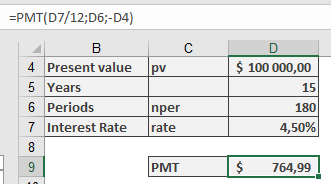
A 60-year-old has $100,000 saved and wants monthly payments for 15 years at 4.5% annual interest.

Scenario A: Exhaust all capital

=PMT(4.5%/12, 15*12, -100000)

Result: $764.99 per month

Scenario B: Maintain $10,000 balance

=PMT(4.5%/12, 15*12, -100000, 10000)

Result: $725.99 per month

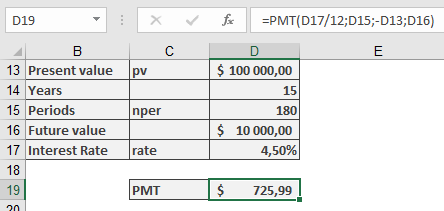
Note: Negative Pv indicates outgoing payment (capital invested)

2. Loan Repayment Calculation

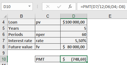
$100,000 loan at 5.5% annual interest with 5-year term and $80,000 residual balance.

=PMT(5.5%/12, 5*12, 100000, -80000)

Result: $748.69 per month (negative indicates outgoing payment)

Key Differences:

• Savings calculations assume compound interest
• Mortgage loans typically use simple monthly interest (annual rate/12)

Important Notes

1. For loans, payments are negative (cash outflow)
2. Interest rates should match payment periods (annual rate/12 for monthly payments)
3. Type parameter significantly affects beginning/end of period calculations
4. Results are theoretical for accounts without true compound interest

Its calculates the yield of a fixed-interest security with an irregular final interest period (different length from previous regular periods), using simple interest (no compounding).

Syntax

ODDLYIELD(Settlement; Maturity; Last_Interest_Date; Rate; Price; Repayment; Frequency; [Basis])

Arguments

Parameter	Requirement	Description
Settlement	Required	Date of bond ownership transfer
Maturity	Required	Date of principal repayment
Last_Interest_Date	Required	Date of last regular interest payment before purchase
Rate	Required	Nominal annual interest rate (coupon rate)
Price	Required	Bond price as percentage of par value (par = 100)
Repayment	Required	Redemption value percentage (per 100 par value)
Frequency	Required	Annual payment frequency (1, 2, or 4)
[Basis]	Optional	Day-count convention (0-4, default=0)

Validation Rules

1. Date Handling:
   • Time values are ignored (truncated)
   • Invalid dates return #NUM! error
   • Required sequence: Maturity > Settlement > Last_Interest_Date
2. Numerical Requirements:
   • Rate ≥ 0, Price ≥ 0 (else #NUM!)
   • Frequency ∈ {1,2,4}
   • Basis ∈ {0,1,2,3,4}

Background

This function complements ODDLPRICE(), calculating the effective yield needed to achieve a specified market price. It uses simple yield methodology (no compounding) where:

1. Annual yield is derived from partial period calculations
2. Interest at maturity includes accruals since last payment date
3. Accrued interest is prorated based on time elapsed

Calculation Method

The yield is determined by:

• Solving the price formula for yield
• Annualizing partial period results
• Prorating interest between last payment and settlement

Example

Sample files demonstrate calculation for bonds with irregular final periods:

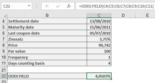
Error Conditions

Error	Trigger Condition
#NUM!	Invalid dates, negative values, or parameter constraints violated
#VALUE!	Non-numeric arguments

Note

Function is only applicable during the final irregular period before maturity.

Its calculates the price of a fixed-interest security with a final interest period that differs in length from previous regular periods, without considering compound interest.

Syntax

ODDLPRICE(Settlement; Maturity; Last_Interest_Date; Rate; Yield; Repayment; Frequency; [Basis])

Arguments

• Settlement (required): Date when ownership of the bond transfers to buyer
• Maturity (required): Date when principal repayment occurs
• Last_Interest_Date (required): Date of last regular interest payment
• Rate (required): Bond’s nominal annual interest rate (coupon rate)
• Yield (required): Market interest rate for bonds of equivalent duration
• Repayment (required): Redemption value as percentage of par value (where par = 100)
• Frequency (required): Interest payments per year (1=annual, 2=semi-annual, 4=quarterly)
• Basis (optional): Day-count convention (see Table 15-2). Defaults to 0 if omitted.

Notes

1. Date inputs must not include time values; decimal places are truncated
2. Frequency and Basis are converted to integers
3. Invalid dates return #NUM! error
4. Rate and Yield must be non-negative; otherwise returns #NUM!
5. Returns #NUM! if:
   • Frequency is not 1, 2, or 4
   • Basis is outside 0-4 range
   • Chronological order is violated: Maturity > Settlement > Last_Interest_Date

Background

The function applies the financial principle:
Creditor’s Payment = Debtor’s Payment

At transaction initiation:

• Security price + accrued interest = Present value of future cash flows
• Price is expressed as percentage of par value (100 units)

Calculation is straightforward when:

• Settlement coincides with interest payment date, and
• Interest is paid annually

Complexities arise when:

• Settlement occurs between interest dates, or
• Multiple annual payments exist

Common financial methods for partial periods include:

• Moosmüller
• Braess/Fangmeyer
• ISMA (see PRICE() and YIELD() background for Excel-ISMA correlation)

Calculation Method

Excel uses simple yield (no compounding) with these principles:

1. Accrued interest calculated from days since last interest payment
2. Partial yield derived from days to maturity (based on year length)
3. Only applicable during final period before maturity

Example

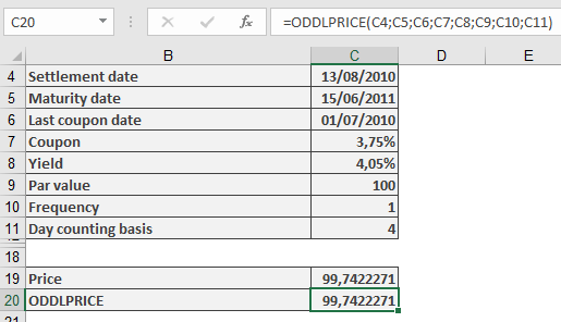
Sample files include a fictitious bond calculation matching the logic, demonstrating:

• Terms with irregular final period
• Price calculation methodology
• Identical results to ODDLPRICE() function output

Its calculates the yield of a fixed-interest security from the settlement date to maturity, accounting for a first interest period that may be shorter or longer than subsequent regular periods.

Syntax

ODDFYIELD(Settlement; Maturity; Issue; First_Interest_Date; Rate; Price; Repayment; Frequency; [Basis])

Arguments

• Settlement (required) – The date the bond is transferred to the buyer.
• Maturity (required) – The date the bond’s principal is repaid.
• Issue (required) – The issuance date of the security.
• First_Interest_Date (required) – The date of the first interest payment.
• Rate (required) – The bond’s nominal annual interest rate (coupon rate).
• Price (required) – The bond’s price at settlement (as a percentage of par value, where par = 100).
• Repayment (required) – Redemption value per 100 units of par value.
• Frequency (required) – Interest payments per year (1 = annual, 2 = semi-annual, 4 = quarterly).
• Basis (optional) – Day-count convention. Defaults to 0 if omitted.

Notes

• Dates must be entered without time values; decimals are truncated.
• Frequency and Basis are truncated to integers.
• Invalid dates return #VALUE!.
• Price and Yield must be non-negative; otherwise, #NUM! is returned.
• If Frequency is not 1, 2, or 4, or Basis is outside 0–4, #NUM! is returned.
• Chronological order must be:
  Maturity > First_Interest_Date > Settlement > Issue; otherwise, #NUM! is returned.

Background

For theoretical details, refer to the ODDFPRICE() function background.

ODDFYIELD() computes the effective yield required for a bond to reach its market price, informing investors of the expected return. The calculation mirrors ODDFPRICE() but solves for yield instead of price.

Example

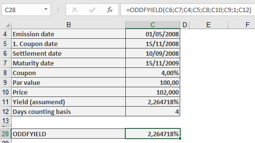
The sample files include a fictitious bond with a shortened first interest period, The yield is derived iteratively (via goal-seek) to match the target price. ODDFYIELD() returns identical results.

Calculates the price of a fixed-interest security, accounting for a first interest period that is either shorter or longer than subsequent regular periods (quarterly, semi-annual, or annual).

Syntax

ODDFPRICE(Settlement; Maturity; Issue; First_Interest_Date; Rate; Yield; Repayment; Frequency; [Basis])

Arguments

• Settlement (required) – The date the security is transferred to the buyer.
• Maturity (required) – The date the security’s principal is repaid.
• Issue (required) – The issuance date of the security.
• First_Interest_Date (required) – The date of the first interest payment.
• Rate (required) – The bond’s nominal annual interest rate (coupon rate).
• Yield (required) – The market yield for bonds of the same maturity.
• Repayment (required) – The redemption value per 100 units of par value.
• Frequency (required) – Number of interest payments per year (1 = annual, 2 = semi-annual, 4 = quarterly).
• Basis (optional) – Day-count convention . Defaults to 0 if omitted.

Notes

• Dates must be entered without time values; decimals are truncated.
• Frequency and Basis are truncated to integers.
• If dates are invalid, #VALUE! is returned.
• Yield and Repayment must be non-negative; otherwise, #NUM! is returned.
• If Frequency is not 1, 2, or 4, or Basis is outside 0–4, #NUM! is returned.
• The chronological order must be:
  Maturity > First_Interest_Date > Settlement > Issue; otherwise, #NUM! is returned.

Background

The function applies the financial principle:

Creditor’s Payment = Debtor’s Payment

At the transaction’s start, the security’s price plus accrued interest equals the present value of future cash flows (interest + principal). The price is expressed as a percentage of par (e.g., 100 units).

Calculating present value is straightforward if:

• The settlement coincides with an interest payment date, and
• Interest is paid annually.

However, complexities arise with:

• Settlement between interest dates, or
• Multiple annual payments.

Finance mathematics uses various methods (e.g., Moosmüller, Braess/Fangmeyer, ISMA) to handle partial periods. For ISMA compatibility with Excel, see the PRICE() and YIELD() background notes.

Formula (Simplified Case)

For annual payments (360-day year) and a shortened first period, the formula in Excel Help reduces to:

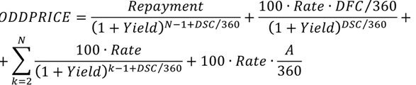
Formula variables:

• N = Total interest periods,
• A = Days from issue to settlement,
• DSC = Days from settlement to first interest date,
• DFC = Days from first interest date to maturity.]

Unlike PRICE(), the first period is treated separately (not summed with others) because its coupon is partial.

For Frequency > 1, Rate and Yield are adjusted for intra-year periods.

For lengthened first periods, the formula accounts for hypothetical interim interest payments realized at the period’s end. Accrued interest is handled similarly.

Note: The function is irrelevant once the first interest date passes.

Example

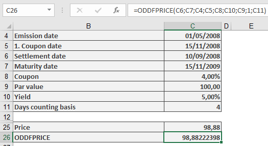
The sample files include a fictitious bond calculation with a shortened first interest period. The result aligns with ODDFPRICE()‘s output.

This function calculates the net present value of future period surpluses (cash flows) of an investment based on a given discount rate.

Syntax

NPV(Rate; Value1; Value2; …)

Arguments

• Rate (required) – The discount rate supplied by the investor.
• Value1, Value2, … (required) – The (actual and expected) surpluses from disbursements and deposits, listed in a continuous column. Each value represents the end of a period (typically one year) in ascending order without gaps. Negative surpluses are indicated with a minus sign.

If the cells in the Value argument contain non-numeric data or are empty, Excel treats them as if they do not exist. This also applies if cell references in the argument point to such cells.

Background

Dynamic investment appraisal methods rely on estimated and projected deposits and disbursements and their yields, unlike static methods, which focus on costs and earnings. Both cash inflows and outflows are evaluated using a uniform discount rate derived from the investor’s experience. The sum of all discounted period surpluses is called the net present value (NPV).

An investment is considered financially viable if the NPV is non-negative, meaning the invested capital plus the expected yield is recovered.

The first value in the NPV() function represents the end of the first period. The net present value of an investment is determined by subtracting the initial disbursement (at the start of the first period) from the result of NPV().

Example

When reviewing the following examples, compare them to the explanations for IRR() and its related examples.

Investment in Material Assets

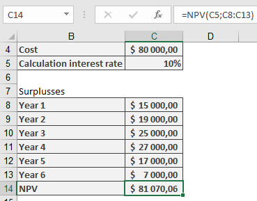
The purchase cost of a machine is $80,000.00. The expected annual surpluses (deposits minus disbursements) are estimated as shown in Table 1.

Table 1. Estimated Annual Surpluses from Machine Usage

Year	Surplus (in $)
1	15,000
2	19,000
3	25,000
4	27,000
5	17,000
6	7,000

Is the investment economically sound if a discount rate of 10% p.a. is applied?

To answer this, enter the purchase cost in the first cell and list the surpluses from Table 1 in a continuous column. Using NPV() returns approximately $81,070, slightly exceeding the purchase cost. Thus, the yield is likely marginally better than the expected rate.

Note: Decimal precision may not be critical when dealing with real investments where future surpluses are estimates.

Financial Investment

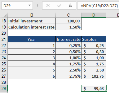
German federal savings bonds (Type A) with the terms as of August 30, 2010 (Table 2) may appear to offer a total yield of around 1.5% at first glance.

Table 2. Terms for Federal Savings Bonds

Duration Year	Nominal Interest
2010/2011	0.25%
2011/2012	0.50%
2012/2013	1.00%
2013/2014	1.75%
2014/2015	2.50%
2015/2016	2.75%

Sample calculations (available in the function’s example files) show that the net present value for a $100.00 investment is only $99.63. Therefore, investing at this expected yield is not advisable.

The NPER() function calculates the duration of a compound interest process, annuity calculation, or repayment plan. It is based on regular payments of the same amount and/or one-time payments at the beginning or end of the period, following the financial mathematical benefit principle:

Payment of the creditor+Payment of the debtor=0Payment of the creditor+Payment of the debtor=0

Syntax:

NPER(Rate, Pmt; Pv; Fv; Type)

Arguments:

• Rate (required) – The (constant) periodic interest rate, expressed as an arrears rate.
• Pmt (required/optional, see Note) – The amount of regular payments (e.g., an annuity).
• Pv (required/optional, see Note) – The present (starting) value of one payment direction.
  • For disbursement plans, this is the initial account balance.
  • For repayment plans, this is the loan amount.
• Fv (optional/required, see Note) – The desired future value (e.g., a residual balance or final repayment amount).
• Type (optional) – Specifies payment timing:
  • 0 or omitted: Payments at the end of each period (default).
  • 1: Payments at the beginning of each period.

Background:

The five financial functions—

• PV() (present value),
• FV() (future value),
• PMT() (regular payment),
• NPER() (number of periods),
• RATE() (interest rate)

—are interrelated through the benefit principle equation, where M represents the payment timing (Type).

The present value and periodic payments are compounded, and the sum is compared to the future value. Each function solves for one variable in this equation when the others are known. For RATE(), an approximation method is used.

Examples:

The following examples illustrate common financial applications.

1. Compound Interest Calculation

An investor deposits $10,000 at a 4.5% annual interest rate, aiming for $25,000. How long must the money remain invested?

=NPER(4.5%, , -10000, 25000)

Result: 20.82 years (the target is exceeded after 21 years).

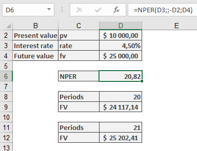
• Verify using FV(4.5%, 20, , -10000) → $24,117.14 (not reached).
• FV(4.5%, 21, , -10000) → $25,202.41 (achieved).

Key Notes:

• For Pmt, Pv, and Fv, ensure at least one is provided (or the calculation is trivial).
• Negative/positive values indicate cash flow direction (outflow vs. inflow).
• Type adjusts the compounding timing for accuracy.