Votre panier est actuellement vide !
Catégorie : Excel function
How to use the COUNT() function in Excel
This function counts the number of numeric entries in an argument list. The COUNT() function tallies cells containing numbers within a specified range or array.
Syntax
COUNT(value1; [value2]; …)Arguments
- value1(required): The first item, cell reference, or range to count
- value2,…(optional): Additional items, cell references, or ranges to count (up to 255 total arguments, or 30 in Excel 2003 and earlier)
Only numeric values are counted; text, logical values, or empty cells are ignored.
Background
While simple in function, COUNT() provides significant time savings, particularly when working with large datasets. Manual counting in extensive tables would be impractical and error-prone.Example
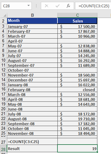
Figure below displays sales data from January 2007 through November 2008 entered by sales representatives.As sales manager, you use COUNT(C3:C25) to determine how many months saw sales activity over this two-year period. The function returns 19, indicating sales occurred in 19 of the 23 months.
How to use the CORREL() function in Excel
This function returns the correlation coefficient of a two-dimensional random variable with values in the cell ranges array1 and array2. Use the correlation coefficient to determine the relationship between two properties.
For example, you can examine the relationship between the number of website visits and online orders.
Syntax
CORREL(array1; array2)Arguments
- array1 (required): A cell range of values.
- array2 (required): A second cell range of values.
Background
Is there any correlation between two variables? This question often arises when analyzing or interpreting data. To answer it, you can use correlation analysis.The correlation coefficient measures the relationship between two properties, producing a value between -1 (perfect negative correlation) and 1 (perfect positive correlation). The sign indicates the direction of the correlation.
Correlation analysis is a key method for determining the linear relationship between two variables (e.g., website visits and online orders).
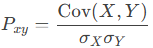
The formula for the correlation coefficient is:
where:
- −1≤Pxy≤1−1≤Pxy≤1
- Cov(X,Y) is the covariance between variables X and Y
- σX and σY are the standard deviations of X and Y
Interpretation
The following guidelines apply to the correlation coefficient:- < 0.3: Weak correlation
- 0.3 – 0.5: Moderate correlation
- 0.5 – 0.7: Distinct correlation
- 0.7 – 0.9: Strong correlation
- > 0.9: Very strong correlation
Example
A software company sells all its products through its website. The company sends newsletters to inform customers about new products and drive traffic to the site.Last year, online orders increased significantly. Management wants to determine whether this growth resulted from marketing efforts or increased website visits.
Using CORREL(), the company analyzes the relationship between website visits and online orders (see Figure below).
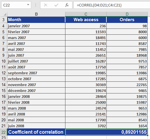
Figure below illustrates the dependency between website visits and orders without the correlation coefficient.
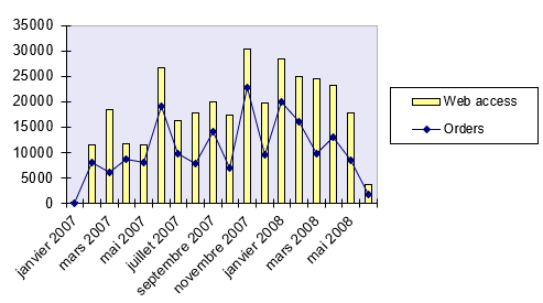
The calculated correlation coefficient of 0.89 indicates a strong positive correlation—meaning that as website visits rise (due to marketing), online orders also increase.
How to use the CONFIDENCE.T() function in Excel
This function returns the confidence interval for the expected value of a random variable using a Student’s *t*-distribution.
Syntax
CONFIDENCE.T(alpha; standard_dev; size)Arguments
- alpha(required): The significance level used to calculate the confidence interval. The confidence level is 100*(1 – alpha)%, meaning an alpha of 05 corresponds to a 95% confidence level.
- standard_dev(required): The standard deviation of the population. This value is assumed to be known.
- size(required): The sample size.
Background
Refer to the background information for the CONFIDENCE.NORM() function.Example
See the example for the CONFIDENCE.T function below.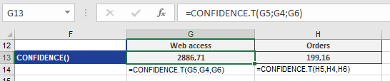
How to use the CONFIDENCE.NORM() function in Excel
This function calculates the margin of error for a confidence interval around a sample mean, assuming a normal distribution and a known population standard deviation. The confidence interval is:
Confidence Interval=xˉ±CONFIDENCE.NORM()
where:
- xˉ = Sample mean.
- The interval has a 100×(1−α)%100×(1−α)% confidence level (e.g., 95% for α=0.05α=0.05).
Syntax
CONFIDENCE.NORM(alpha; standard_dev; size)
Arguments
Argument Required? Description alpha Yes Significance level (e.g., 0.05 for 95% confidence). Must be between 0 and 1. standard_dev Yes Population standard deviation (must be known). size Yes Sample size (must be > 1). Background
- Key Concepts:
- Confidence Interval: A range where the true population mean is likely to fall.
- Margin of Error: CONFIDENCE.NORM() returns half the width of this range.
- Assumptions:
- Data is normally distributed.
- Population standard deviation (σσ) is known.
- Formula:
Margin of Error=zα/2×σnMargin of Error=zα/2×nσ
-
- zα/2zα/2 = Critical value from the standard normal distribution (e.g., 1.96 for 95% confidence).
- σ = Population standard deviation.
- n = Sample size.
- Interpretation:
- A 95% confidence interval means:
« If we repeated this experiment 100 times, ~95 of the calculated intervals would contain the true population mean. »
- A 95% confidence interval means:
Example: Website Traffic Analysis
Scenario
A software company analyzes monthly website visits and orders over 4 years (n=43n=43 months):
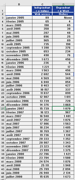
- Sample mean (xˉxˉ): 11,308.11 visits/month.
- Population standard deviation (σσ): 9,500 (assumed known).
- Confidence level: 95% (α=0.05α=0.05).
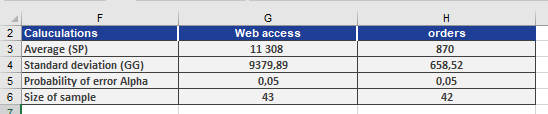
Step 1: Calculate Margin of Error
CONFIDENCE.NORM(0.05, 9500, 43) // Returns 2,803.57
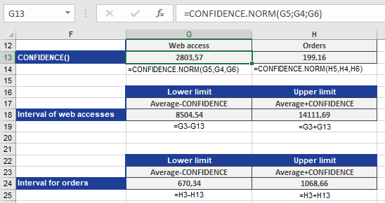
Step 2: Construct Confidence Interval
11,308.11±2,803.57=[8,504.54, 14,111.69]11,308.11±2,803.57=[8,504.54, 14,111.69]
Conclusion
- 95% Confidence Interval: [8,504.54, 14,111.69] visits/month.
- Interpretation: We are 95% confident the true population mean of monthly visits lies in this range.
Key Notes
- When to Use:
- Estimating population means when σ is known (rare in practice; consider CONFIDENCE.T() if σ is unknown).
- Quality control, market research, or any scenario requiring precision estimates.
- Limitations:
- Inaccurate for small samples: Requires n≥30n≥30 for reliable results unless data is perfectly normal.
- Misinterpretation Risk: A 95% CI does not mean there’s a 95% chance the true mean is in the interval (it’s fixed).
- Common Errors:
- #NUM! if:
- α≤0α≤0 or ≥1≥1.
- size≤1size≤1.
- #VALUE! if non-numeric inputs are provided.
- #NUM! if:
How to use the CHISQ.INV.RT() function in Excel
This function returns the inverse of the right-tailed chi-square (χ²) distribution, providing the critical value where:
- If probability = CHISQ.DIST.RT(x, df), then CHISQ.INV.RT(probability, df) = x.
Syntax
CHISQ.INV.RT(probability; degrees_freedom)
Purpose
Used in hypothesis testing to:
- Determine critical values for χ² tests (e.g., goodness-of-fit, independence).
- Validate whether observed results significantly deviate from expected results under the null hypothesis.
Arguments
Argument Required? Description probability Yes Right-tailed probability (α) associated with the χ²-distribution (e.g., 0.05 for 5% significance). degrees_freedom Yes Degrees of freedom (positive integer). For contingency tables: (rows – 1) * (columns – 1). Background
- Right-Tailed χ² Distribution:
- Models the sum of squared deviations from expected values.
- Used when testing « greater than » hypotheses (e.g., variance exceeds a threshold).
- Key Concepts:
- Critical Value (x):
- The χ² value beyond which the null hypothesis is rejected.
- Calculated as CHISQ.INV.RT(α, df).
- Degrees of Freedom (df):
- Depends on the test type. For a 2×2 contingency table, df = 1.
- Critical Value (x):
- Inverse Relationship:
- CHISQ.INV.RT(α, df) is the inverse of CHISQ.DIST.RT(x, df).
Example: Vitamin C Efficacy Study
Scenario
- Goal: Test if Vitamin C reduces cold risk (null hypothesis: no effect).
- Data:
- Expected cold cases (no Vitamin C): 22/936.
- Observed cold cases (Vitamin C group): Fewer than 22.
- Significance Level (α): 2.5% (one-tailed test).
Step 1: Calculate Critical Value
CHISQ.INV.RT(0.025; 1) // Returns 5.0239
- Interpretation: If the test statistic (v) > 5.0239, reject the null hypothesis.

Step 2: Compute Test Statistic (v)
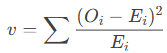
- For each category, calculate:
-
- Oi = Observed frequency.
- Ei = Expected frequency.
- Result: Suppose v = 6.47 (see Figure below).
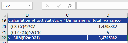
Step 3: Compare v to Critical Value
- 6.47 > 5.0239 → Reject the null hypothesis.
- Conclusion: Insufficient evidence to confirm Vitamin C reduces colds at α = 2.5%.
Key Notes
- When to Use:
- Goodness-of-Fit Tests: Compare observed vs. expected frequencies.
- Independence Tests: Check if two categorical variables are related.
- Degrees of Freedom:
- For a contingency table: df = (rows – 1) * (columns – 1).
- For variance tests: df = sample size – 1.
- Common Errors:
- #NUM! if:
- probability ≤ 0 or ≥ 1.
- degrees_freedom < 1.
- #NUM! if:
How to use the CHISQ.TEST() function in Excel
This function performs a chi-square (χ²) test of independence, returning the p-value associated with the test statistic. It compares observed frequencies (actual_range) against expected frequencies (expected_range) to determine if there is a statistically significant association between categorical variables.
Syntax
CHISQ.TEST(actual_range; expected_range)
Arguments
Argument Required? Description actual_range Yes Range of observed frequencies (e.g., survey counts). expected_range Yes Range of expected frequencies under the null hypothesis. Note:
- Ranges must have the same dimensions. If not, #N/A is returned.
- Expected frequencies should ideally be ≥5 for reliable results.
Background
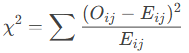
- Chi-Square Test Statistic (χ²):
-
- Oij = Observed frequency in row ii, column jj.
- Eij= Expected frequency (calculated from row/column totals).
- Degrees of Freedom (df):
- For an r×cr×c contingency table:
df=(r−1)(c−1)df=(r−1)(c−1)
- Null Hypothesis (H₀):
- Assumes no association between variables (observed ≈ expected).
- Low p-value (e.g., <0.05): Reject H₀ (significant association).
Example: Vitamin C and Colds Study
Scenario
- Goal: Test if Vitamin C usage affects cold incidence.
- Data:
- Observed (actual_range): 22 colds in 936 Vitamin C users.
- Expected (expected_range): 30 colds (baseline rate without Vitamin C).
Step 1: Run CHISQ.TEST()
CHISQ.TEST(A2:A3; B2:B3) // Returns p-value = 0.01 (1%)
*(See Figure below for setup.)*
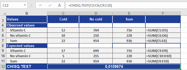
Step 2: Interpret Results
- p-value = 0.01:
- 1% probability that the deviation (observed vs. expected) is due to chance.
- Conclusion: Reject H₀ at 99% confidence (Vitamin C likely reduces colds).
Key Outputs
Metric Value Interpretation χ² Statistic Calculated Higher = greater deviation. Degrees of Freedom 1 (2×2 table: (2-1)(2-1)=1). p-value 0.01 Significant at α=0.05. Key Notes
- When to Use:
- Goodness-of-fit: Compare observed vs. theoretical distributions.
- Independence tests: Check if two categorical variables are related (e.g., gender vs. product preference).
- Limitations:
- Small expected frequencies: May violate test assumptions (use Fisher’s Exact Test if any Eij<5Eij<5).
- Binary outcomes: For 2×2 tables, consider Yates’ correction for continuity.
- Follow-up Analysis:
- If significant, calculate Cramer’s V or Phi coefficient to measure association strength.
How to use the CHISQ.INV() function in Excel
This function returns the inverse of the left-tailed chi-squared (χ²) distribution.
- Given a probability (cumulative probability), it finds the corresponding χ² value (x) such that:
- If probability = CHISQ.DIST(x; df; TRUE), then CHISQ.INV(probability; df) = x.
- Used to determine critical values for hypothesis testing (e.g., goodness-of-fit tests).
Syntax
CHISQ.INV(probability; degrees_freedom)
Arguments
Argument Required? Description probability Yes A cumulative probability (0 ≤ probability < 1). degrees_freedom Yes Degrees of freedom (positive integer). Background
- Inverse Chi-Squared Distribution:
- Solves for x in:
P(X≤x)=probabilityP(X≤x)=probability
-
- Where:
- P = Cumulative probability (area under the left tail).
- x = Chi-squared statistic.
- Where:
- Left-Tailed vs. Right-Tailed:
- CHISQ.INV(): Left-tailed inverse (returns the χ² value for a given cumulative probability).
- CHISQ.INV.RT(): Right-tailed inverse (returns the χ² value for 1 – probability).
- Key Applications:
- Hypothesis Testing: Find critical values to reject/fail to reject the null hypothesis.
- Confidence Intervals: Calculate bounds for variance estimates.
Example
The CHISQ.DIST() function is the inverse function of CHISQ.INV().

Key Notes
- Degrees of Freedom (df):
- Determines the shape of the χ² distribution. For a contingency table, df = (rows – 1) * (columns – 1).
- Common Use Cases:
- Goodness-of-Fit Tests: Compare observed vs. expected frequencies (e.g., Mendel’s pea experiments).
- Independence Tests: Check if two categorical variables are related.
- Error Handling:
- Returns #NUM! if:
- probability ≤ 0 or ≥ 1.
- degrees_freedom < 1.
- Returns #NUM! if:
- Given a probability (cumulative probability), it finds the corresponding χ² value (x) such that:
How to use the BINOM.INV() function in Excel
This function returns the minimum number of successes (k) in a binomial distribution where the cumulative probability is ≥ a specified threshold (alpha). It is the inverse of BINOM.DIST().
Syntax
BINOM.INV(trials; probability_s; alpha)
Key Use Case:
- Quality Control: Determine the maximum allowable defective items in a batch before rejecting it.
- Decision-Making: Find critical thresholds for pass/fail scenarios (e.g., survey results, manufacturing tolerances).
Arguments
Argument Required? Description trials Yes Total number of independent trials (e.g., 100 surveys). probability_s Yes Probability of success per trial (e.g., 0.5 for 50%). alpha Yes Target cumulative probability threshold (e.g., 0.95 for 95% confidence). Background
- Inverse Binomial Distribution:
- Solves for k in:
P(X≤k)≥αP(X≤k)≥α
-
- Where:
- P = Cumulative binomial probability.
- k = Maximum successes allowed before exceeding the threshold.
- Where:
- Assumptions:
- Trials are independent (e.g., coin flips, quality checks).
- Only two outcomes per trial (success/failure).
- Relation to BINOM.DIST():
- If BINOM.DIST(k, n, p, TRUE) = alpha, then BINOM.INV(n, p, alpha) = k.
Example: Vacation Survey
Scenario:
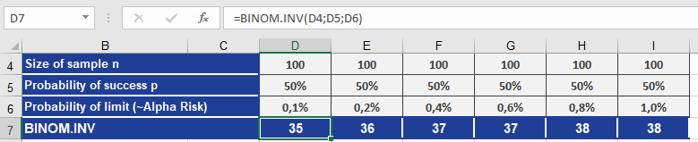
- You ask 100 people for directions, each with a 50% chance (p = 0.5) of answering « yes. »
- Question: What is the maximum number of « yes » responses (k) where the cumulative probability ≤ 0.1% (alpha = 0.001)?
Formula:
BINOM.INV(100, 0.5, 0.001)
Result: 35 (see Figure below).
Interpretation:
- There is a 0.1% chance that 35 or fewer people would say « yes » by random chance.
- If you observe >35 « yes » answers, the result is statistically significant (exceeds the threshold).
Key Notes
- Quality Control Application:
- If a batch of 1,000 parts has a 2% defect rate (p = 0.02), use BINOM.INV() to find the maximum defects allowed before rejecting the batch (e.g., for alpha = 0.95).
- Threshold Logic:
- Lower alpha = Stricter criteria (fewer allowed successes).
- Higher alpha = More lenient criteria (more allowed successes).
- Limitations:
- For large trials (e.g., >1,000), consider approximations like the Normal distribution.
How to use the BINOM.DIST() function in Excel
This function calculates probabilities for a binomial distribution, which models scenarios with:
- A fixed number of trials (trials).
- Only two outcomes per trial: success or failure.
- Independent trials with a constant success probability (probability_s).
Syntax
BINOM.DIST(number_s; trials; probability_s; cumulative)
Example Use Case:
- Calculating the probability that 50 out of 100 people support a smoking ban, given each has a 60% chance of supporting it.
Arguments
Argument Required? Description number_s Yes Number of successful trials (e.g., 50 « yes » responses). trials Yes Total number of trials (e.g., 100 surveys). probability_s Yes Probability of success per trial (e.g., 0.6 for 60%). cumulative Yes TRUE = Cumulative probability (≤ number_s successes).
FALSE = Exact probability (exactly number_s successes).Background
- Binomial Distribution Basics:
- Models counts of successes in n independent Bernoulli trials (e.g., coin flips, survey responses).
- Probability Mass Function (PMF):

-
-
- (nk)(kn) = Combination of n trials with k successes (COMBIN(n, k) in Excel).
- p = Success probability per trial.
-
- Key Properties:
- Mean (Expected Value): μ=n×pμ=n×p
- Variance: σ2=n×p×(1−p)σ2=n×p×(1−p)
- Bernoulli Process:
- Named after mathematician Jakob Bernoulli.
- Each trial is independent with outcomes 1 (success) or 0 (failure).
Examples
- Vacation Directions (Yes/No Survey)
Problem:
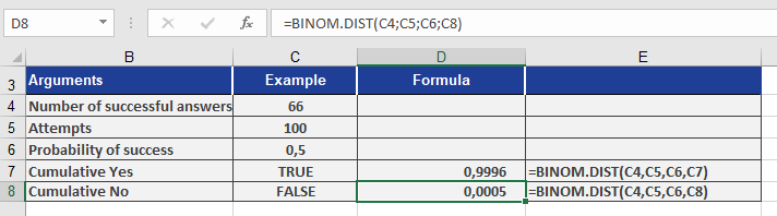
- You ask 100 strangers for directions, with a 50% chance (p = 0.5) each says « yes. »
- What’s the probability that exactly 66 answer « yes »?
Formula:
BINOM.DIST(66; 100; 0.5; FALSE) // Exact probability
Result: 0.05% (see Figure below).
Cumulative Probability (≤66 yes answers):
BINOM.DIST(66, 100, 0.5, TRUE) // Returns ~100%
- Damaged Packages (Quality Control)
Problem:
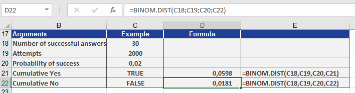
- A factory produces 2,000 packages, with a 2% defect rate (p = 0.02).
- What’s the probability that exactly 30 are damaged?
Formula:
BINOM.DIST(30; 2000; 0.02; FALSE) // Exact probability
Result: 1.8% (see Figure below).
Cumulative Probability (≤30 damaged):
BINOM.DIST(30; 2000; 0.02; TRUE) // Returns 6%
Key Notes
- When to Use:
- FALSE: For exact counts (e.g., « What’s the chance of exactly 3 wins in 5 games? »).
- TRUE: For thresholds (e.g., « What’s the chance of ≤3 wins? »).
- Assumptions:
- Trials must be independent (e.g., survey responses don’t influence each other).
- probability_s must stay constant across trials.
- Limitations:
- For large trials (e.g., >1000), consider approximations like the Poisson or Normal distribution.
How to use the BETA.INV() function in Excel
This function returns the inverse of the beta cumulative distribution. Given a probability, it finds the corresponding value x such that:
- If probability = BETA.DIST(x, …), then BETA.INV(probability, …) = x.
Syntax
BETA.INV(probability; alpha; beta; [A]; [B])
Common Use Case:
- In project planning, it estimates completion times based on expected duration and variance.
Arguments
Argument Required? Description probability Yes A probability (0 ≤ probability ≤ 1) linked to the beta distribution. alpha Yes Shape parameter (must be > 0). beta Yes Shape parameter (must be > 0). A No Lower bound (default = 0). B No Upper bound (default = 1). Note: If A is specified, B must also be provided.
Background
- Beta Distribution Basics:
- Models continuous probabilities for variables bounded in [0, 1].
- Defined by shape parameters alpha (p) and beta (q).
- Probability Density Function :

-
-
- B(p, q) = Beta function (normalization factor).
- Γ(p) = Gamma function.
-
- Key Properties:
- Expected Value: E[X] = alpha / (alpha + beta)
- Variance: Var(X) = (alpha * beta) / [(alpha + beta)^2 * (alpha + beta + 1)]
- Inverse Function:
- BETA.INV() reverses BETA.DIST(), returning the quantile x for a given probability.
Example
Problem:
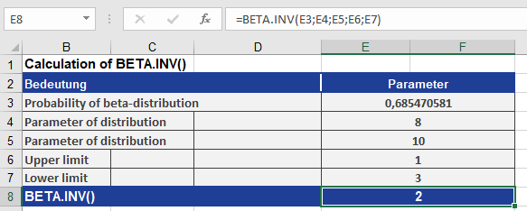
- Given a beta distribution with:
- Shape parameters: alpha = 8, beta = 10
- Bounds: A = 1, B = 3
- What value x corresponds to a cumulative probability of 0.68547?
Formula:
BETA.INV(0.685470581, 8, 10, 1, 3)
Result: 2 (see Figure below).
Interpretation:
- There is a 68.547% probability that a random variable from this distribution falls below 2 (within the range [1, 3]).
Key Notes
- Bounds Adjustment:
- If A and B are provided, the result scales linearly from [0, 1] to [A, B].
- Applications:
- Project Management: Estimating task durations (PERT analysis).
- Statistics: Modeling proportions (e.g., conversion rates, survey responses).
- Error Handling:
- Returns #NUM! if probability ≤ 0 or ≥ 1, or if alpha/beta ≤ 0.