Votre panier est actuellement vide !
Catégorie : Excel function
How to use the TRANSPOSE function in Excel
The TRANSPOSE function is used to switch the orientation of a given range or array – converting vertical ranges to horizontal and vice versa.
Syntax:
=TRANSPOSE(array)
Argument:
- array (Required):
The range of cells to be transposed. When transposed:- The first row becomes the first column of the new array
- The second row becomes the second column
- This pattern continues for all rows/columns
USING THE TRANSPOSE FUNCTION
Example: Convert Vertical Range to Horizontal
Original Vertical Range (A1:B5)
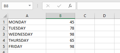
Steps to Transpose:
- Select blank cells in a horizontal arrangement matching the original range’s dimensions (e.g., 2 columns × 5 rows → select 5 columns × 2 rows)
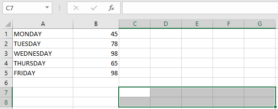
- Enter the formula:
=TRANSPOSE(A1:B5)
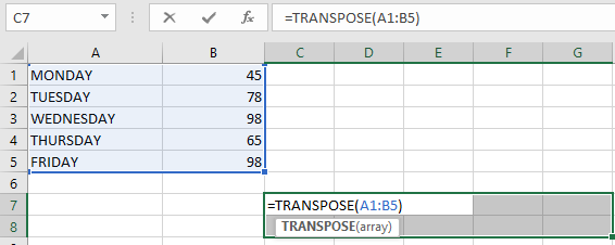
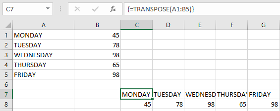
- Press Ctrl+Shift+Enter (to enter as an array formula)
Result:
IMPORTANT NOTES:
- Array Formula Requirement:
- Must be entered with Ctrl+Shift+Enter (not just Enter)
- Curly braces {} will appear around the formula
- Editing Restrictions:
- Cannot modify part of the transposed array
- To edit: Select entire transposed range → Make changes → Re-apply with Ctrl+Shift+Enter
- Range Dimensions:
- Target range must have inverse dimensions of source range
- (e.g., 3 rows × 2 columns → needs 2 rows × 3 columns blank cells)
- Dynamic Arrays (Excel 365):
- Newer versions don’t require Ctrl+Shift+Enter
- Automatically spills results
- array (Required):
How to use the MATCH function in Excel
The MATCH function is used to search for a specified value within a range of cells and returns the relative position of that value within the range.
Syntax:
=MATCH(lookup_value; lookup_array; [match_type])
Arguments:
- lookup_value (Required):
- The value you want to find within the lookup_array.
- lookup_array (Required):
- The range of cells being searched.
- match_type (Optional):
- Specifies how Excel matches the lookup_value with values in the lookup_array.
match_type Behavior 1 or omitted Finds the largest value ≤ lookup_value. Requires lookup_array to be sorted in ascending order. 0 Finds the first exact match. Does not require sorting. -1 Finds the smallest value ≥ lookup_value. Requires lookup_array to be sorted in descending order. USING THE MATCH FUNCTION
Example: Find the Position of « Apple »
Given the following table:
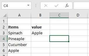
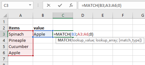
- Select an empty cell and enter
=MATCH(B3; A3:A6; 0)
(Where B3 contains « Apple »)
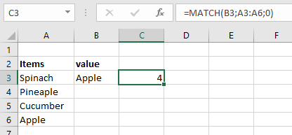
- Press Enter → Returns 4 (Apple is the 4th item in the range).
NOTES & ERRORS
- Case-Insensitive: Does not distinguish uppercase/lowercase.
- #N/A Error: Occurs if no match is found.
- Wildcards Supported: Use * (any sequence) or ? (single character) for partial matches.
- Exact vs. Approximate: Use match_type=0 for exact matches; 1 or -1 for approximate (requires sorted data).
- lookup_value (Required):
How to use the CHOOSE function in Excel
The CHOOSE function selects and returns a value from a list based on a specified index number.
The syntax for the CHOOSE function is as follows:
=CHOOSE(index_num; value1; [value2]; …)
Arguments:
- index_num (Required):
- An integer between 1 and 254 that indicates which value to return.
- Can be a number, formula, or cell reference.
- value1, value2, … (value1 required, others optional):
- A list of up to 254 values from which CHOOSE selects.
- Values can be numbers, text, formulas, cell references, or defined names.
USING THE CHOOSE FUNCTION
Consider the following list of names in cells A2:A5:
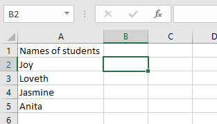
Example: Return the 3rd Value (Jasmine)
- Select an empty cell and enter:
=CHOOSE(3; A2; A3; A4; A5)
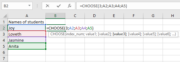
- Press Enter—the function returns Jasmine (the 3rd value).
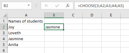
NOTES & ERROR HANDLING
- Text values must be in quotes, or Excel returns #NAME?.
- #VALUE! Error occurs when:
- index_num is <1 or >number of values provided.
- index_num is non-numeric (e.g., text).
- index_num (Required):
How to use the HLOOKUP function in Excel
The HLOOKUP function (where « H » stands for Horizontal) is used to search for a specific value in the top row of a table or dataset and retrieve corresponding data from another row in the same column.
The syntax for the HLOOKUP function is as follows:
=HLOOKUP(lookup_value; table_array; row_index_num; [range_lookup])
Arguments:
- lookup_value (Required): The value to search for in the first row of the table.
- table_array (Required): The range of cells containing the data to be searched.
- row_index_num (Required): The row number (within the table array) from which to return the matching value.
- range_lookup (Optional): Specifies whether to find an exact match (FALSE) or an approximate match (TRUE).
- If TRUE (or omitted), it finds the closest match (or next largest value if no exact match exists).
- If FALSE, it returns an exact match or #N/A if no match is found.
USING THE HLOOKUP FUNCTION
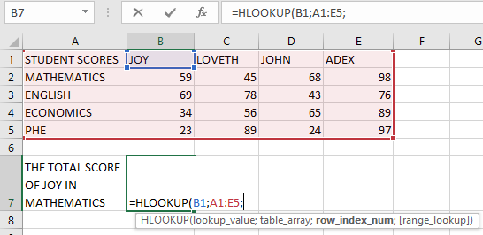
Consider the following example table containing student names and their scores in different subjects. We will use HLOOKUP to find Joy’s score in Mathematics.
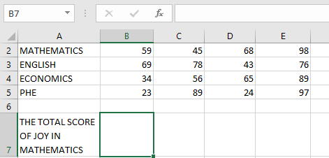
Steps to Find Joy’s Math Score:
- Select an empty cell and begin the HLOOKUP function with the lookup_value (e.g., cell B1 containing « Joy »):
=HLOOKUP(B1;
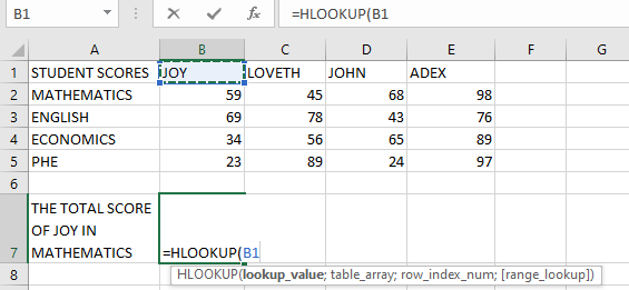
- Define the table_array (the range where data is stored, e.g., A1:E5):
=HLOOKUP(B1; A1:E5;
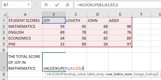
- Specify the row_index_num (the row containing the return value, e.g., 3 for « Math »):
=HLOOKUP(B1; A1:E5; 3;
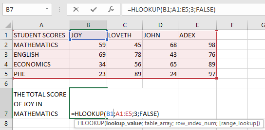
- Choose between exact or approximate match (use FALSE for exact, TRUE for approximate):
=HLOOKUP(B1; A1:E5; 3; FALSE)
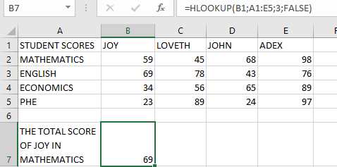
- Press Enter, and the result should be 59 (Joy’s Math score).
NOTES WHEN USING THE HLOOKUP FUNCTION
- Like VLOOKUP, HLOOKUP is not case-sensitive (treats « JOY » and « joy » the same).
- Wildcards (*, ?, ~) can be used for partial matches.
- Only the first matching value is returned if duplicates exist.
Common Errors:
- #N/A! → No match found when range_lookup is FALSE.
- #REF! → Occurs if row_index_num exceeds the table’s row count.
- #VALUE! → Occurs if:
- row_index_num is less than 1.
- Non-numeric row_index_num is provided.
How to use the VLOOKUP function in Excel
The VLOOKUP function (where « V » stands for Vertical) is used to quickly search for a specific value in the first column of a table or dataset and retrieve corresponding data from another column in the same row.
The syntax for the VLOOKUP function is as follows:
=VLOOKUP(lookup_value; table_array; col_index_num; [range_lookup])
Arguments:
- lookup_value (Required): The value to search for in the first column of the table.
- table_array (Required): The range of cells containing the data to be searched.
- col_index_num (Required): The column number (within the table array) from which to return the matching value.
- range_lookup (Optional): Specifies whether to find an exact match (FALSE) or an approximate match (TRUE).
- If TRUE (or omitted), it finds the closest match (or next largest value if no exact match exists).
- If FALSE, it returns an exact match or #N/A if no match is found.
USING THE VLOOKUP FUNCTION
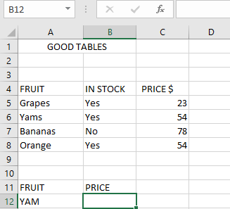
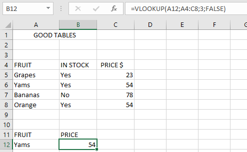
Consider the following example table containing 4 fruits and their prices. We will use VLOOKUP to find the price of Yam.
Steps to Find the Price of Yam:
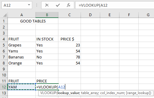
- Select an empty cell and begin the VLOOKUP function with the lookup_value (e.g., cell A12 containing « Yam »):
=VLOOKUP(A12;
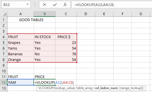
- Define the table_array (the range where data is stored, e.g., A4:C8):
=VLOOKUP(A12; A4:C8,
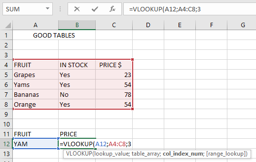
- Specify the col_index_num (the column containing the return value, e.g., 3 for « Price »):
=VLOOKUP(A12; A4:C8; 3
- Choose between exact or approximate match (use FALSE for exact, TRUE for approximate):
=VLOOKUP(A12; A4:C8; 3; FALSE)
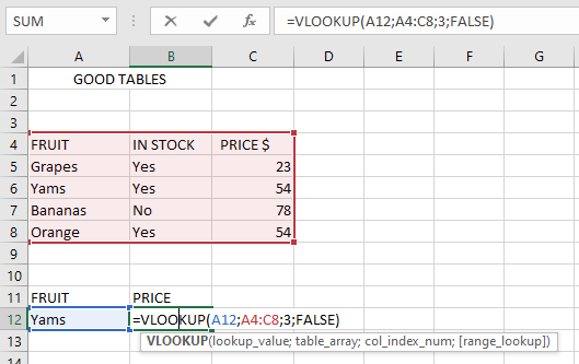
- Press Enter, and the result should be 54 (the price of Yam).
NOTES WHEN USING THE VLOOKUP FUNCTION
- If range_lookup is omitted, VLOOKUP defaults to TRUE (approximate match).
- If duplicate values exist, VLOOKUP returns only the first match.
- VLOOKUP is not case-sensitive (treats « APPLE » and « apple » the same).
- Wildcards (*, ?, ~) can be used for partial matches.
Common Errors:
- #N/A! → No match found for the lookup value.
- #VALUE! → Occurs if:
- col_index_num is less than 1 or non-numeric.
- range_lookup is not TRUE/FALSE.
- #REF! → Happens when:
- col_index_num exceeds the table’s column count.
- A referenced cell in the formula does not exist.
How to use the MEDIAN function in Excel
The MEDIAN function calculates the middle value of a given set of numbers. For example, the function returns 3 in =MEDIAN(1;2;3;4;5).
The MEDIAN function contains the following arguments:
=MEDIAN(number1; [number2]; …)
Number1 (Required Argument): The range of one or more cells containing values for median calculation.
Number2 (Optional Argument): Additional numbers to include (up to 255 arguments).USING THE MEDIAN FUNCTION
Using the table below, let’s calculate the median of numeric data: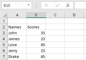
- Select an empty cell and enter:
=MEDIAN(B3:B7)
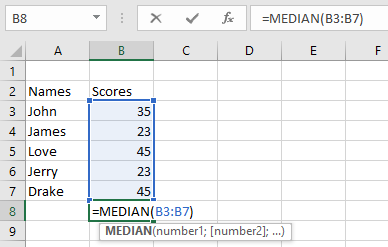
- Press Enter – the result will be 35 (as shown below).

NOTE: Important MEDIAN function behaviors:
- Returns errors if arguments contain uninterpretable text/errors
- Accepts numbers, named ranges, arrays, or number-containing references
- Ignores empty cells, logical values, and text entries
- For even-numbered sets: returns average of two middle values
How to use the MAX function in Excel
The MAX function returns the maximum or largest number in a given set of values or arguments. The MAX function ignores text and logical values in its calculations.
The MAX function uses the following argument:
=MAX(number1; [number2]; …)
Number1 (Required Argument): This is the range of cells from which the highest number will be returned.
Number2 (Optional Argument): Here, up to 255 additional numbers can be included.USING THE MAX FUNCTION
With the table given below, find the maximum number using the MAX function.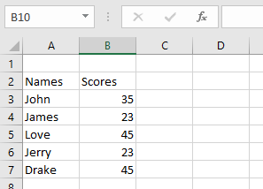
To find the maximum number using the MAX function, follow the steps below:
- Select an empty cell and type in the function name and its arguments:
=MAX(B3:B7)
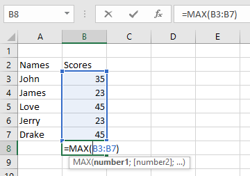
- Click Enter and the result will be 45 as shown in the table below.
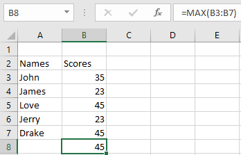
NOTE: Keep these in mind when using the MAX function:
- A #VALUE! error occurs when non-numeric values are provided
- The MAX function returns 0 for arguments without numbers
- To include logical values and text representations of numbers, use the MAXA function
- Arguments can be numbers, names, arrays, or references containing numbers
- Empty cells, logical values, and text are ignored
- Error values or uninterpretable text in arguments will cause errors
How to use the MIN function in Excel
The MIN function returns the smallest numeric value from a given set of values. The function ignores text entries and logical values (TRUE/FALSE) in its calculations.
The MIN function uses the following syntax:
=MIN(number1; [number2]; …)
Number1 (Required Argument): The first number, cell reference, or range containing numeric values to evaluate.
Number2,… (Optional Argument): Additional numbers or ranges to include (up to 255 total arguments).USING THE MIN FUNCTION
Using the table below, we’ll find the smallest number with the MIN function.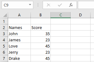
To determine the minimum value:
- Select an empty cell and enter:
=MIN(B3:B7)
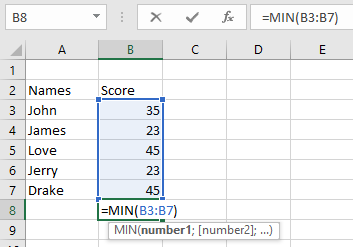
- Press Enter to display the result: 23 (as shown below).
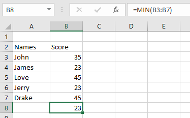
NOTE: Important MIN function behaviors:
- Returns #VALUE! error if non-numeric data is provided
- To evaluate logical values and text-formatted numbers, use MINA instead
- Accepts numbers, named ranges, arrays, or number-containing references
- Automatically ignores:
- Empty cells
- Text entries
- Logical values
- Returns 0 for arguments without valid numbers
- Returns errors when arguments contain:
- Uninterpretable text
- Error values
How to use the AVERAGEIFS function in Excel
The AVERAGEIFS function calculates the average (arithmetic mean) of cells that meet multiple specified criteria. This function supports logical operators (<, >, <>) and wildcards (*, ?) in its criteria and was introduced in Excel 2007.
The AVERAGEIFS function uses the following syntax:
=AVERAGEIFS(average_range; criteria_range1; criteria1; [criteria_range2; criteria2]; …)
Average_range (Required): The range of cells to average (containing numbers, names, arrays, or numeric references).
Criteria_range1 (Required): The first range to evaluate against criteria1.
Criteria1 (Required): The condition for criteria_range1 (number, expression, cell reference, or text).
Criteria_range2, criteria2,… (Optional): Additional ranges (up to 127) and their corresponding criteria.USING THE AVERAGEIFS FUNCTION
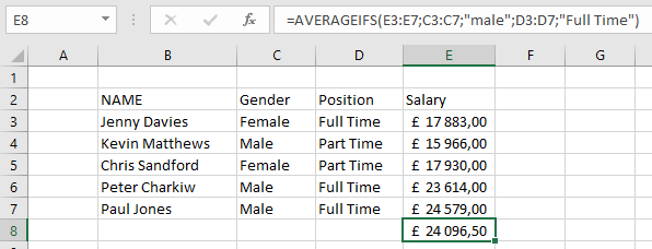
Let’s calculate the average salary of full-time male employees from the table below.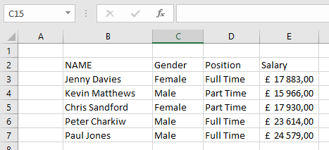
To find this average:
- Select an empty cell and enter:
=AVERAGEIFS(E3:E7; C3:C7; « Male »; D3:D7; « Full Time »)
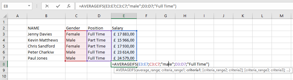
- Press Enter to display the result: £24 096,50 (as shown below).
NOTE: Key points about AVERAGEIFS:
- Empty criteria ranges are treated as zero
- All criteria ranges must match average_range in size
- Numbers/dates with logical operators must be quoted (e.g., « >4/23/2018 »)
- TRUE/FALSE values evaluate as 1/0 respectively
- #DIV/0! error occurs when:
- average_range is empty or contains text
- values can’t be interpreted numerically
- no cells meet all criteria
- Supports wildcards (*, ?) in criteria
How to use the AVERAGEIF function in Excel
The AVERAGEIF function calculates the average of cells that meet specified criteria. This function supports logical operators (<, >, <>, =) and wildcards (*, ?) in its criteria.
The AVERAGEIF function uses the following syntax:
=AVERAGEIF(range; criteria; [average_range])
Range (Required Argument): The set of cells to evaluate, which may contain numbers, names, arrays, or number-containing references.
Criteria (Required Argument): The condition determining which cells to average (can be a number, expression, cell reference, or text – e.g., 13, « <14 »).
Average_range (Optional Argument): The actual cells to average. If omitted, the function uses the range argument.USING THE AVERAGEIF FUNCTION
Let’s calculate the average sales of cakes from the table below.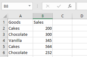
To find the average sales of chocolate cakes:
- Select an empty cell and enter:
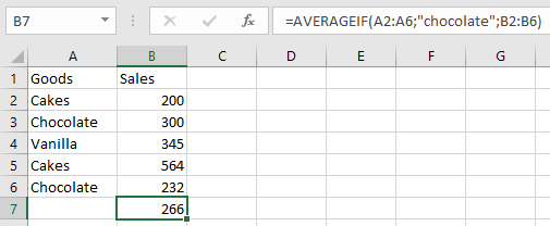
=AVERAGEIF(A2:A6; « chocolate »; B2:B6)

- Press Enter to display the result: 266 (as shown below).
NOTE: Important AVERAGEIF considerations:
- #DIV/0! error occurs when:
- No cells meet the criteria
- The range is empty or contains text
- Criteria referencing empty cells are treated as zero
- Cells with TRUE/FALSE values are ignored
- Supports wildcards (*, ?) in criteria