Étiquette : date and time function

It is use to calculates the number of working days between two dates while excluding:

• Custom-defined weekends (not limited to Saturday/Sunday)
• Specified holidays

Syntax

NETWORKDAYS.INTL(start_date, end_date, [weekend], [holidays])

Arguments

• start_date (required): First day of the period.
• end_date (required): Last day of the period.
• weekend (optional): Defines non-working days. Options:
  • Number codes (1-7, 11-17): Predefined weekend combinations (see table below).
  • 7-digit string: Custom weekly off-days (e.g., « 0000011 » = Saturday/Sunday).
  • Default: 1 (Saturday/Sunday off).
• holidays (optional): Additional non-working dates (cell range or array).

Weekend Codes Reference

Number	Weekend Days	String Equivalent
1 (default)	Saturday, Sunday	« 0000011 »
2	Sunday, Monday	« 1000001 »
3	Monday, Tuesday	« 1100000 »
4	Tuesday, Wednesday	« 0110000 »
5	Wednesday, Thursday	« 0011000 »
6	Thursday, Friday	« 0001100 »
7	Friday, Saturday	« 0000110 »
11	Sunday only	« 0000001 »
12	Monday only	« 1000000 »
…	…	…
17	Saturday only	« 0000010 »

Note: Strings use 1 for off-days and 0 for workdays (e.g., « 0101000 » = Monday/Wednesday off).

Example

 Assume that a project is planned from December 12, 2008, through June 2, 2009. You have to calculate the number of workdays in this timeframe, excluding holidays. The formula

=NETWORKDAYS.INTL(« 12/12/10″, »06/02/11 »,1,

{« 12/25/10″, »01/01/11″, »01/17/11 », »02/21/11 « , »05/30/2011″, »07/04/11 »})

returns 121 workdays for the project. Note that in the formula, holidays are enclosed in braces and not in parentheses.

Notes

• Error Handling: Returns #VALUE! for invalid dates or text entries.
• Flexibility: Supports any weekend pattern except « 1111111 » (no workdays).
• Pro Tip: Name your holiday range (e.g., Holidays) for cleaner formulas.

The NETWORKDAYS function is use to calculates the number of working days between two dates, automatically excluding:

• Weekends (Saturday & Sunday)
• Custom holidays (if specified)

Syntax

NETWORKDAYS(start_date, end_date, [holidays])

Arguments

• start_date (required): First day of the period.
• end_date (required): Last day of the period.
• holidays (optional):
  • A range of cells containing holiday dates
  • An array of serial numbers (e.g., {« 1/1/2023 », « 12/25/2023 »})

Example

 Assume that a project is planned to extend over the period from December 12, 2008, through June 2, 2009. You have to calculate the number of workdays in this timeframe, excluding holidays. The formula

=NETWORKDAYS(« 12/12/10″, »06/02/11 »,

{« 12/25/10″, »01/01/11″, »01/17/11″, »02/21/11 », « 05/30/2011″, »07/04/11 »})

returns 121 workdays for the project. Note that in the preceding formula, holidays are enclosed in braces and not in parentheses. The table below  shows the calculation using cell references for the start date, end date, and holidays.

Key Features

• Inclusive Counting: Both start_date and end_date are counted if they are workdays.
• Holiday Handling: Excludes dates listed in the holidays argument.
• Error Cases: Returns #VALUE! for invalid dates or text entries.

Notes

• Alternative: Use NETWORKDAYS.INTL() for custom weekends (e.g., Friday-Saturday weekends).
• Tip: Name your holiday range (e.g., Holidays) for easier reference.
• Error Handling:

=IFERROR(NETWORKDAYS(Start, End, Holidays), « Check dates ») 

Its extracts the month number (1-12) from a date, where:

• 1 = January
• 12 = December

Syntax

MONTH(serial_number)

Arguments

• serial_number (required):
  • A valid date
  • Can be:
    • A date string (e.g., « 11/14/1959 »)
    • A serial number (Excel date format)
    • A cell reference containing a date
    • The result of another function (e.g., TODAY())

Background

Part of Excel’s date function family (with YEAR() and DAY()). Used to:

• Extract months for grouping/sorting data
• Support monthly reporting
• Enable date-based calculations

Examples

 Assume that you want to enable the Excel AutoFilter for the months and need to calculate the month values from a date column by using an auxiliary column. To do this, use the formula

=MONTH(date_value)

Here are more examples:

Formula	Returns	Explanation
=MONTH(TODAY())	9 (if current month is September)	Current month number
=MONTH(« 11/14/1959 »)	11	November extraction
=MONTH(« 01/01/1900 »)	1	January extraction
=MONTH(« 12/31/1899 »)	#VALUE!	Invalid date (pre-1900 in Windows)
=MONTH(« 12/31/9999 »)	#VALUE!	Invalid
=MONTH(« 01/01/10000 »)	#VALUE!	Invalid date (post-9999)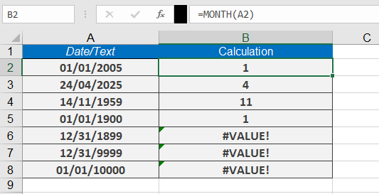

Notes

• Returns #VALUE! for:
  • Text-formatted dates
  • Dates outside Excel’s valid range (1/1/1900–12/31/9999 for Windows)
• Combine with YEAR() and DAY() for complete date analysis

The MINUTE function is use to extracts the minute component from a time value (with or without an associated date). Returns an integer between 0 and 59.

Syntax

MINUTE(serial_number)

Arguments

• serial_number (required):
  • A valid time value
  • Can be entered as:
    • A time string in quotes (e.g., « 06:43 »)
    • A decimal number representing time (e.g., 0.27986111 for 06:43)
    • The result of another formula/function (e.g., NOW())
    • A cell reference containing a time/date

Background

Part of Excel’s time function family (along with HOUR() and SECOND()). Used to:

• Extract minute values for time-based calculations
• Analyze scheduling data
• Build dynamic time-dependent formulas

Example

 Assume that you need to calculate the minutes after the full hours.

Here are example formulas:

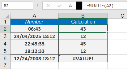
=MINUTE(« 06:43 ») returns 43 minutes.

=MINUTE(« 12/24/2010 18:12 ») returns 12.

=MINUTE(NOW()) returns the current minute.

Notes

• Returns #VALUE! for invalid time formats
• For decimal inputs:
  • 0.0 = 12:00:00 AM
  • 0.5 = 12:00:00 PM
  • 0.999 = 11:59:59 PM
• Combine with HOUR() and SECOND() for complete time extraction

This function is essential for time tracking, scheduling, and data analysis in Excel.

Its extracts the hour component from a time value (with or without an associated date). Returns an integer between 0 (midnight) and 23 (11 PM).

Syntax

HOUR(serial_number)

Arguments

• serial_number (required):
  • A valid time value
  • Can be entered as:
    • Time string in quotes (e.g., « 06:43 »)
    • Decimal number representing time (e.g., 0.27986111 for 06:43)
    • Result of other formulas/functions
    • Cell reference containing time/date

Background

Part of Excel’s time function family (along with MINUTE() and SECOND()). Used to:

• Extract hour components for calculations
• Analyze time-based data
• Create time-dependent formulas

Example

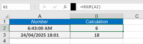
If you want to extract the hours from a time value, you can use the formula

=HOUR(« 06:43 »)

which returns 6 hours.

Here are some more examples:

=HOUR(« 24/04/2025 18:01 ») returns 18.

=HOUR(NOW()) returns the current hour.

Notes

• Returns #VALUE! for invalid time formats
• For decimal inputs:
  • 0.0 = 12:00 AM
  • 0.5 = 12:00 PM
  • 0.999 = 11:59 PM
• Combine with MINUTE() and SECOND() for complete time breakdown

Its returns the serial number representing the last day of the month, calculated as a specified number of months before or after a given start date;

Syntax

EOMONTH(start_date, months)

Arguments

• start_date (required):
  • The initial date for calculation
  • Can be a date string, serial number, or reference to a cell containing a date
• months (required):
  • Integer value specifying the number of months to add (positive) or subtract (negative)
  • Decimal values are truncated (e.g., 2.9 becomes 2)

Background

Primarily used in financial applications for:

• Calculating payment due dates
• Determining maturity dates
• Setting month-end reporting periods

Alternative Calculation Method:

=DATE(YEAR(start_date), MONTH(start_date) + months + 1, 1) – 1

This formula:

1. Advances to the first day of the month after the target month
2. Subtracts one day to get the last day of the target month

Error Handling

• Returns #NUM! error if:
  • start_date is invalid or text-formatted
  • Resulting date falls outside Excel’s valid date range (1/1/1900 to 12/31/9999 for Windows)

Examples

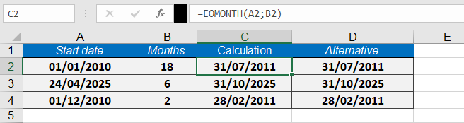
Assume that you want to designate the last day of the month as the due date for a credit period 18 months from January 1, 2010. The formula

=EOMONTH(« 01/01/2010 »,18)

returns 07/31/2011 as the due date as seen bellow

This function is particularly valuable for financial professionals who need to calculate precise month-end dates for various accounting and reporting purposes.

The EDATE function is use to Returns the serial number of the date that is a specified number of months before or after a given start date.

Syntax

EDATE(start_date, months)

Arguments

• start_date (required): The initial date for the calculation.
• months (required): The number of months to add (positive) or subtract (negative).

Background

• Calculates future or past dates by adding/subtracting months while preserving the day value (unless invalid for the new month).
• Alternative method using DATE(), YEAR(), MONTH(), and DAY():

=DATE(YEAR(start_date), MONTH(start_date) + months, DAY(start_date)) 

• Errors:
  • #VALUE! if start_date is invalid.
  • Non-integer months are truncated (e.g., 3.9 becomes 3).

Examples

 Assume that you want to calculate the end of months of 4 construction project. The formula given bellow;

Formula	Result	Notes
=EDATE(« 01/02/2010 », 18)	07/02/2011	18 months later
=EDATE(« 01/02/2010 », 24)	01/02/2012	2 years later (24 months)
=EDATE(« 01/03/2010 », 0)	01/03/2010	Same date (months=0)
=EDATE(« 01/04/2010 », -5)	08/04/2009	5 months earlier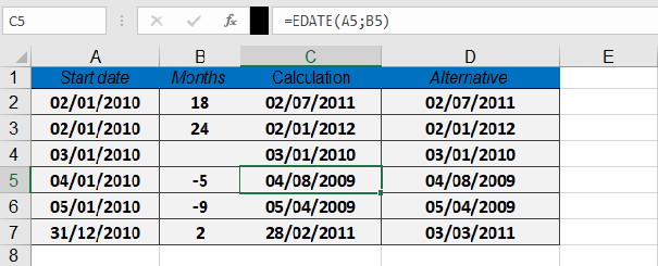

Key Notes

• Day Adjustment: If the resulting month has fewer days (e.g., =EDATE(« 31/01/2023 », 1)), Excel returns the last valid day (February 28 or 29).
• Formatting: Apply date formatting to display the serial number as a readable date.

The DAYS360 is use to calculates the number of days between two dates based on a 360-day year (12 months × 30 days each), commonly used in financial and accounting calculations.

Syntax

DAYS360(start_date, end_date, [method])

Arguments

• start_date (required): The beginning date of the period.
• end_date (required): The ending date of the period.
• method (optional): Specifies the calculation method:
  • FALSE or omitted: U.S. (NASD) method
    • If the start date is the last day of a month, it is treated as the 30th of the same month.
    • If the end date is the last day of a month:
      • If the start date is before the 30th, the end date becomes the 1st of the next month.
      • Otherwise, the end date becomes the 30th of the same month.
  • TRUE: European method
    • Any 31st of a month is treated as the 30th of the same month.

Background

• Primarily used for interest calculations in financial applications (e.g., bonds, loans).
• Returns a negative number if start_date > end_date.
• Always use the Excel percent format for interest rates (e.g., 5.25%).

Interest Calculation Formula

To compute interest over a period:

Interest = Capital × Interest Rate × DAYS360(start_date, end_date, [method]) / 360

Use ROUND() to format the result to 2 decimal places (currency format).

Example

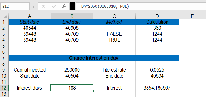
Calculate interest for $250,000 at 5.25% from November 22, 2010 (cell C12) to May 31, 2011 (cell E12):

1. Calculate Days (European method):

=DAYS360(C12, E12, TRUE) 

Returns: 188 days.

1. Compute Interest:

=C11 * E11 * DAYS360(C12, E12, TRUE) / 360 

Returns: $6,854.17.

Key Notes

• Error Handling: Ensure dates are valid (use IFERROR for robustness).
• Method Selection: Choose TRUE (European) or FALSE (U.S.) based on financial standards.

The DAY function extracts and returns the day number (1-31) from a given date.

Syntax

DAY(serial_number)

Arguments

• serial_number (required): The date value from which to extract the day. Can be:
  • A cell reference containing a date
  • A date serial number
  • A date entered as text in Excel-recognized format

Background

• Part of Excel’s date function family (along with YEAR() and MONTH())
• Extracts the day component for use in calculations or data analysis
• Works with Gregorian calendar dates only
• Returns #VALUE! error for invalid dates

Key Points

1. Date Systems:
   • Windows (1900 system): Valid dates 1/1/1900 to 12/31/9999
   • Mac (1904 system): Valid dates 1/1/1904 to 12/31/9999
2. Error Conditions:
   • Dates outside valid range return #VALUE!
   • Text that can’t be interpreted as a date returns #VALUE!
3. Practical Applications:
   • Extracting days for filtering or grouping
   • Date-based calculations
   • Data validation

Examples

Formula	Result	Notes
=DAY(« 07/13/2008 »)	13	Standard date format
=DAY(« 11/14/1959 »)	14	Day extraction
=DAY(« 01/01/1900 »)	1	Earliest valid date in Windows system
=DAY(« 12/31/1899 »)	#VALUE!	Before valid date range
=DAY(« 12/31/9999 »)	31	Latest valid date
=DAY(« 01/01/10000 »)	#VALUE!	Beyond valid date range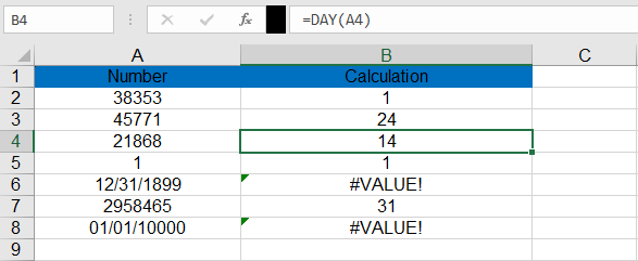

Note: For error handling with potentially invalid dates:

=IFERROR(DAY(A2), »Invalid Date »)

Converts a date stored as text into a serial number that Excel recognizes as a date.

Syntax

DATEVALUE(date_text)

Arguments

• date_text (required): A text string representing a date in any valid Excel date format.

Background

• Essential for converting imported or text-formatted dates into numeric values for calculations.
• While Excel often auto-converts text dates, DATEVALUE() ensures reliability with:
  • Imported data
  • Third-party add-in outputs
  • Non-standard date formats

Key Features

1. Date Systems:
   • Windows (1900 system): Accepts dates from 1/1/1900 to 12/31/9999
   • Mac (1904 system): Accepts dates from 1/1/1904 to 12/31/9999
   • Out-of-range dates: Return #VALUE! error
2. Partial Dates:
   • Missing year: Uses current system year
   • Missing day: Defaults to 1st of month
   • Time values: Always ignored
3. Format Flexibility:
   • Supports multiple text date formats (MM/DD/YYYY, DD-MM-YYYY, Month YYYY, etc.)

Examples

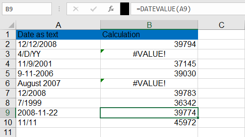
Formula	Result (Windows)	Notes
=DATEVALUE(« 12/12/2008 »)	39794 (displays as 12/12/2008)	Full date conversion
=DATEVALUE(« 11/11 »)	11/11/[current year]	Auto-fills current year
=DATEVALUE(« August 2007 »)	08/01/2007	Month-year becomes 1st of month
=DATEVALUE(« 2008/11/22 »)	11/22/2008	Handles YYYY/MM/DD format

as shown below;

Note: Combine with error checking for imported data:

=IFERROR(DATEVALUE(A2), « Invalid Date »)