Étiquette : lookup and reference function

This function searches for a value in the leftmost column of a table and returns a value from the same row in a specified column. The range_lookup argument determines whether an exact or approximate match is required.

Syntax

VLOOKUP(lookup_value; table_array; col_index_num;[range_lookup])

Arguments

• lookup_value (required)
  Can be text, a number, or a logical value. This is the value to search for in the first column of the table.
• table_array (required)
  A reference to a range of cells or an array constant (numbers and text must be enclosed in braces {}).
• col_index_num (required)
  Must be a positive integer indicating the column number from which to return the value. The leftmost column is 1.
• range_lookup (optional)
  A logical value:
  • TRUE (or omitted): Finds the closest match (approximate).
  • FALSE: Requires an exact match.

Background

• If range_lookup is FALSE, VLOOKUP() searches for an exact match in the first column. If none is found, it returns #N/A. The table does not need to be sorted.
• If range_lookup is TRUE or omitted, the function returns:
  • An exact match if one exists.
  • Otherwise, the largest value less than lookup_value.
  • Note: In this case, the table must be sorted in ascending order to ensure correct results.

Examples

The following examples demonstrate how to use VLOOKUP().

Combining with Other Functions

The INDEX() function can be used with VLOOKUP() to find exact matches.

• VLOOKUP() only retrieves values to the right of the search column.
• For more flexible searches across a table, use INDEX() and MATCH().

Example Scenario:
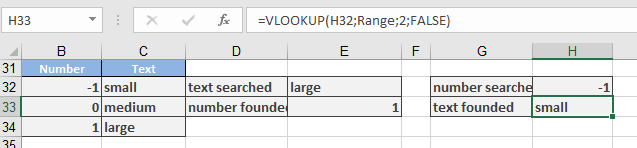
Assume a table (Range = B32:C34) assigns numbers to text (e.g., -1 = small).

1. Finding text from a number:

=VLOOKUP(-1; Range; 2; FALSE) 

Returns « small ».

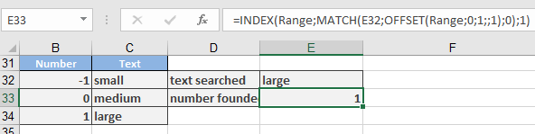
1. Finding a number from text (inverse lookup):

=INDEX(Range; MATCH(F32; OFFSET(Range; 0; 1; ; 1); 0); 1) 

1. • OFFSET() shifts the search to the second column.
   • MATCH() finds the row containing the value in F32.
   • INDEX() retrieves the corresponding value from column 1.

Flips the orientation of a range or array, converting rows to columns and vice versa.

Syntax:

TRANSPOSE(array)

Background. Use TRANSPOSE() as an array formula for a range that includes the same number of rows or columns as the initial array. The rows and columns are exchanged: The rows in the “old” array become the columns in the “new” array. The first row becomes the first column, the second row becomes the second column, and so on.

If you don’t use the necessary number of rows or columns in the destination range, the missing content is truncated. If you use too many rows or columns, the excess cells are filled with the #N/A error. When you use array constants (numbers or text in braces) in the expression

{=TRANSPOSE({11,12,13;21,22,23})}

the argument is interpreted as an array with two rows and three columns, and the result fits into an array with three rows and two columns. In the formula

{=TRANSPOSE({1;2;3;4})}

the argument is a single column that is converted into a row.

Key Features:

• Input: Requires a range (e.g., A1:B3) or array constant (e.g., {1,2;3,4}).
• Output: Returns a reoriented array where:
  • Original rows become columns
  • Original columns become rows
• Dynamic Arrays (Excel 365+): Automatically spills results without Ctrl+Shift+Enter.

Example

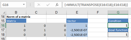
Arrays and vectors are used for calculations in linear algebra, linear optimization, and decision theory. Vectors are always interpreted as column vectors. In this case, the scalar product of two vectors is the array multiplication of the first vector and the second transposed vector. For this purpose, Excel provides the MMULT() function for array multiplications.

• The norm of the n-dimensional square array A can be calculated like this: Calculate the number resulting from the maximum of all scalar products between A and x if x iterates all vectors with the norm, 1 (the root from the scalar product of x with itself).

This is a task for the Solver, an Excel add-in that you must activate. Assume that this three-dimensional array includes B16 through D18. You use a placeholder for all vectors x in E16 through E18 (dynamic cells). You enter the scalar product of x with itself in G16 (a secondary condition):

{=MMULT(TRANSPOSE(E16:E18);E16:E18)}

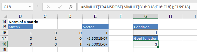
You enter the formula that calculates the scalar product of Ax with x in G18:

=MMULT(TRANSPOSE(MMULT(B16:D18;E16:E18));E16:E18)

Returns the number of rows in a specified array or cell range.

Syntax:

ROWS(array)

Arguments:

Argument	Required?	Description
array	Yes	A cell range (e.g., A1:B5) or array constant (e.g., {1;2;3}).

Key Behavior:

1. Cell Ranges:
   • =ROWS(A1:A10) → Returns 10.
2. Array Constants:
   • =ROWS({1;2;3;4;5;6}) → Returns 2 (rows separated by ;).
3. Errors:
   • #NULL! → If range intersection is empty (e.g., =ROWS(B2:D4 E2:E4)).
   • #REF! → If using discontiguous ranges without proper parentheses.

Examples:

1. Basic Row Count

• Formula:

=ROWS(B2:D10) 

Result: 9 (9 rows in the range).

2. Dynamic Last Cell in a Named Range

• Formula:

=INDEX(MyRange; ROWS(MyRange); COLUMNS(MyRange)) 

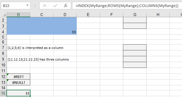
• • How It Works:
    • ROWS(MyRange) → Total rows in MyRange.
    • COLUMNS(MyRange) → Total columns.
    • INDEX retrieves the value at the last row/column intersection.

Returns the row number of a specified cell or range. If no argument is provided, it returns the row number of the cell containing the formula.

Syntax:

ROW([reference])

Arguments:

Argument	Required?	Description
reference	No	A cell or range (e.g., A1, B2:D5). If omitted, defaults to the formula’s cell.

Key Behavior:

1. Single Cell Reference:
   • =ROW(C10) → Returns 10.
2. Range Reference:
   • =ROW(B2:D5) → Returns an array of row numbers {2;3;4;5} (requires Ctrl+Shift+Enter in older Excel).
3. Omitting Reference:
   • If entered in cell F7, =ROW() → Returns 7.

Examples:

1. Generate Consecutive Numbers

• Formula in A15:

=ROW() – ROW($A$15) + 1 & « . »

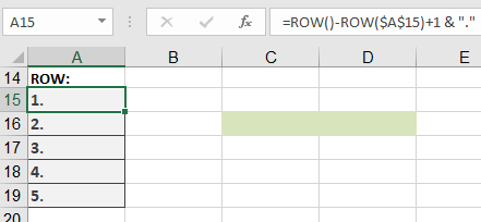
• • Result in A15: 1.
  • Copied down: 2., 3., etc.

2. Dynamic Numbering in a Named Range

• Array Formula (Ctrl+Shift+Enter in legacy Excel):

{=ROW(Range) – ROW(OFFSET(Range, 0, 0, 1)) + 1 & « . »}

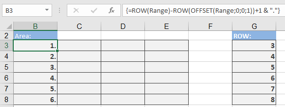
• • How It Works:
    • ROW(Range) → Array of row numbers in the range.
    • ROW(OFFSET(…; 1)) → Gets the first row of the range.
    • Subtracting adjusts numbering to start at 1.

3. Extract Row Number from a Cell

• Formula:

=ROW(INDEX(5:5; 1; 1)) 

• • Result: 5 (returns the row number of row 5).

Common Errors & Fixes:

Error	Cause	Solution
#VALUE!	Non-reference argument (e.g., ROW(« text »)).	Use a valid cell/range reference.
#N/A	Output range larger than input (array formulas).	Match output size to input.

Advanced Uses:

1. Conditional Formatting (Highlight Every 3rd Row)

• Rule Formula:

=MOD(ROW(); 3) = 0 

2. Dynamic Sum Based on Row Position

• Formula:

=SUM(A1:INDEX(A:A; ROW() – 1)) 

• • Sums all cells above the formula’s row.

3. Find Last Used Row in Column A

• Formula:

=MAX(ROW(A:A)*(A:A<> » »)) 

• • Note: Enter with Ctrl+Shift+Enter in legacy Excel.

Comparison with ROWS():

Function	Returns	Example
ROW()	Row number of a cell.	=ROW(A3) → 3
ROWS()	Count of rows in a range.	=ROWS(A1:A10) → 10

 

Returns a dynamic reference to a range shifted by a specified number of rows/columns from a starting cell or range.

Syntax:

OFFSET(reference; rows; cols; [height]; [width])

Arguments:

Argument	Required?	Description
reference	Yes	The anchor cell or range (e.g., A1 or B2:D5). Must be a valid reference.
rows	Yes	Number of rows to offset (positive = down, negative = up).
cols	Yes	Number of columns to offset (positive = right, negative = left).
height	No	Row count of the returned range. Defaults to reference’s height.
width	No	Column count of the returned range. Defaults to reference’s width.

Background. This function doesn’t move cells on the worksheet; it moves the reference to a specified range. If you specify a value for the rows and columns arguments beyond the current sheet, the OFFSET() function returns the #REF! error.

The function expects integers for the four last arguments, and the last two integers must be positive. If the expressions in these arguments are evaluated to fractions, the decimal places are removed. No error occurs.

If you don’t specify the height and width arguments, Excel assumes that the new reference has the same height and width as the initial reference.

If the height argument is smaller than the height of the destination range, the remaining cells display the #N/A error. The same applies to the width argument. If the value is 1, the corresponding rows and columns are repeated in the remaining cells. As shows an example below.

The reference named MyRange has the dimensions two rows x three columns. The formula

{=OFFSET(MyRange;0;1;2;1)}

moves the target to the first cell in the range (B13) and offsets this by zero rows and one column, taking the starting point to cell C13. The height and width parameters extend the range to two rows and one column to target C13:C14. The destination range F13:I15 has the dimensions three rows x four columns. The destination range is filled with the values from C13:C14, repeating this four times across the destination range, but the remaining row

(15) is filled with the error #N/A.

Examples:

The following examples illustrate how the OFFSET() function is used.

 Use this function to address single cells in the original named range. In this case, you don’t move the entire range but only the upper-left corner of the range. If you specify the value 1 for the height and width, the result is a single cell.

Assume that your range, MyRange, includes cells B5 through D6. Cell D6 is the last cell in the range and can be addressed with the array formula

{=OFFSET(MyRange;1;2)}

 To move the required reference to the right or down, start at the upper-left cell of the range: two cells to the right and one cell down.

This method is especially useful if you use dynamic ranges, which change over time (for example, a dynamic list, a manually entered list, or a list updated with a database). In this case, use the COUNT() or COUNTIF() function to specify the position. This is explained in the following examples.

Assume that you have a list like the one shown in the table below. You want to filter the information in the list using database functions. The list constantly changes because records are added or removed.

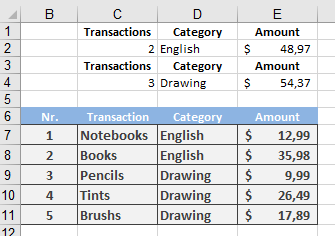
Create the data list in a worksheet named Calculations. The titles of the columns don’t have to match the list titles (for example, you could use Category instead of Categories).

Select the list titles. Select the Insert/Names/Define menu option or click Define Name in the Defined Names group on the

Formula tab. Enter the name list for the range defined by the following formula:

=OFFSET(Calculations!$B$6:$E$6;0;0;COUNT(Calculations!$B:$B)+1)

Based on the number of numeric entries in column B, the upper-left cell of the title range ($B$6:$E$6) is dynamically extended by the adjustable height argument. Remember that +1 is necessary to include the titles in the list.

You can now add up the invoice amounts in the English category using the following formula:

=DSUM(list;E6;D1:D2)

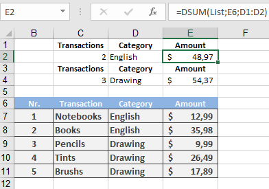
The DSUM() function takes the values identified by the list range and sums the values in the Amount column according to the criteria set in the range D1:D2 (Category, English). Other entries are evaluated with DCOUNT()

=DCOUNT(list;B6;D1:D2)

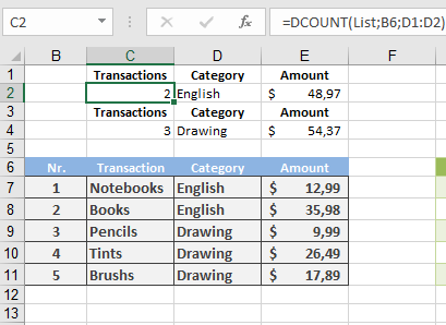
to return a count of the transaction. (The second argument can be empty.)

If you use Excel and format the list as a table, you don’t have to specify the range name. If the table has the name Table1 (the default name), the formula is

=DCOUNT(Table1[#All];B6;D1:D2)

You can use the method explained in the previous example to generate dynamic charts. Define a dynamic range name and use the  named range to create the chart. Use a named range for the legend and data, as in these formulas:

=OFFSET(Charts!$C$4;0;Charts!$B$23)

=OFFSET(Charts!$C$5:$C$19;0;Charts!$B$23)

where the value in cell B23 defines which column should be selected to generate the chart.

Common Errors & Fixes:

Error	Cause	Solution
#REF!	Offset outside sheet limits.	Adjust rows/cols or anchor point.
#N/A	Output range larger than height/width.	Ensure height/width ≥ destination range.
#VALUE!	Invalid reference (e.g., non-range).	Use a cell/range reference (e.g., A1).

Alternatives to OFFSET():

• INDEX() + MATCH(): More efficient for static lookups.
• Excel Tables (Ctrl+T): Auto-expanding ranges without formulas.
• INDIRECT(): For text-based references (but volatile).

Searches for a specified value (lookup_value) within a row, column, or array and returns its relative position (not the value itself).

Syntax:

MATCH(lookup_value; lookup_array; [match_type])

Arguments:

Argument	Required?	Description
lookup_value	Yes	The value to search for (text, number, or logical). Supports wildcards (*, ?) if match_type = 0.
lookup_array	Yes	A single row or column range or array to search.
match_type	No	Determines the match behavior:

• 1 (default): Finds the largest value ≤ lookup_value (requires ascending order).
• 0: Finds the exact match (order irrelevant).
• -1: Finds the smallest value ≥ lookup_value (requires descending order). |

Key Rules & Background:

1. Sorting Requirements:
   • match_type = 1 → Data must be ascending (numbers → text → FALSE/TRUE).
   • match_type = -1 → Data must be descending.
   • match_type = 0 → No sorting needed (exact match).
2. Wildcards (*, ?):
   • Only work with match_type = 0.
   • * = any sequence of characters.
   • ? = any single character.
3. Case Sensitivity:
   • Not case-sensitive (e.g., « APPLE » = « apple »).
4. Errors:
   • #N/A → Value not found or invalid match_type for data.

Examples

The following examples show how this function is used.With the MATCH() function, you can quickly search multiple columns. Assume that you have a price list for clothing as seen below;

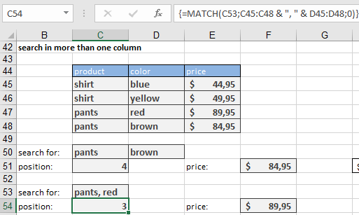
You can determine the position of the yellow shirt with the formula

{=MATCH(C50 & D50;C45:C48 & D45:D48;0)}

Because this is an array formula, you have to press Ctrl+Shift+Enter after entering the formula. The & links elements in the lookup_value and combines the two search columns into one column.

The INDEX() function returns the price:

=INDEX(E45:E48,C51)

Of course, you can combine both formulas into a single formula:

{=INDEX(E45:E48;MATCH(C50 & D50;C45:C48 & D45:D48;0))}

To enter the search criteria in a single row (C53 in Figure 9-9), use the following formula:

{=MATCH(C53;C45:C48 & « ;  » & D45:D48;0)}

This is also an array formula. The search columns are now combined.

You can use the placeholders to find the elements even if you know only part of their names. If you enter pa in C58 and re in D58, the formula

{=MATCH(« * » & C58 & « * » & D58 & « * »;C45:C48 & D45:D48;0)}

finds the row containing the red pants.

Cross tabulations (the simplest form of PivotTable) are often used. These include tables such as time tables, distances between cities, and rate tables. Assume that you have a phone rate comparison table that tells you who the cheapest provider is at certain times of the day. As shows an example below.

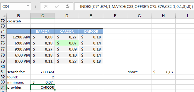
Looking for a time in the left column is a job for MATCH(). But what column contains the result? Use the MATCH() function to find the row, and

the MIN() and OFFSET() functions to find the cheapest rate. Here is the MATCH() function:

=MATCH(C81;B75:B79;1)

And here are the MIN() and the OFFSET() functions:

=MIN(OFFSET(C75:E79;C82-1;0;1;3))

You can combine both formulas into one. Thus, the following formula locates the provider who offers the cheapest rate:

=INDEX(C74:E74;1;MATCH(C83;OFFSET(C75:E79;C82-1;0;1;3);0))

Comparison with Other Functions:

Feature	MATCH()	VLOOKUP()/HLOOKUP()	LOOKUP()
Returns	Position	Value	Value
Exact Match	Yes (with 0)	Yes (with FALSE)	No
Flexibility	High (works with INDEX)	Moderate	Low

Pro Tips:

• Combine with INDEX() for dynamic lookups (superior to VLOOKUP).
• Use match_type = 0 for unsorted data or wildcard searches.
• Avoid #N/A with IFERROR():

=IFERROR(MATCH(…), « Not Found ») 

This function converts a text string into a cell reference or named range.

Syntax:

INDIRECT(reference; [A1])

Arguments:

• reference (required) – A text string that can be interpreted as a valid cell reference (e.g., « A1 », « Sheet1!B5 ») or a named range.
• A1 (optional) – A logical value (TRUE/FALSE) that determines the reference style:
  • TRUE or omitted → Uses A1 notation (e.g., « B2 »).
  • FALSE → Uses R1C1 notation (e.g., « R2C2 » for cell B2).

Background:

• If reference is not a valid cell or range, the function returns #REF!.
• External references (to other workbooks) require the source workbook to be open.

Examples:

1. Using Cell Addresses:
   • Combines with ADDRESS() to convert a generated string into a reference.
   • Example:

=INDIRECT(ADDRESS(2; 3))  // Returns the value in cell C2.

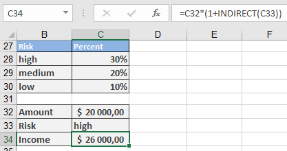
1. Investment Analysis:
   • A simplified model lets users input « high », « medium », or « low » to fetch corresponding yields.
   • Named ranges:
     • high = C28 (e.g., 8%),
     • medium = C29 (e.g., 5%),
     • low = C30 (e.g., 2%).
   • Formula:

=C32 * (1 + INDIRECT(C33)) 

1. • • If C33 contains « high », INDIRECT(C33) fetches the value from C28.
     • With C32 (investment capital) = $1000, the result is $1080 (for 8% yield).

Key Notes:

• Dynamic References: Useful for creating flexible formulas where the target cell changes based on input.

This function retrieves a value (or reference) from an array or cell range based on specified row and column indices.

Syntax (Array Version):

INDEX(array; row_num; [column_num])

Syntax (Reference Version):

INDEX(reference; row_num; [column_num]; [area_num])

Arguments

Array Version:

• array (required): A range of cells or an array constant (e.g., {1,2;3,4}).
• row_num (optional):
  • The row number to return (must be ≤ total rows).
  • Omit if array has only one row.
• column_num (optional):
  • The column number to return (must be ≤ total columns).
  • Omit if array has only one column.

Reference Version:

• reference (required): One or more cell ranges (use parentheses for multiple ranges: (A1:B2, C1:D2)).
• row_num, column_num (optional): Same as array version, but can reference non-contiguous areas.
• area_num (optional): Selects which range in reference to use (e.g., 1 for the first range).

Background

Array Version:

• Indices start at 1.
• Omitting row_num or column_num returns an entire column/row (use as an array formula).
• Errors:
  • #REF! if indices exceed the range.
  • #VALUE! if omitting arguments in non-array formulas.

Reference Version:

• Use parentheses for multiple ranges (e.g., (A1:B2, C1:D2)).
• area_num selects the nth range (default: 1).

Examples

1. Basic Array Usage:

• Return a single value:

=INDEX(B4:C6, 3, 2)  // Returns C6 (3rd row, 2nd column). 

• Array constant (columns separated by commas, rows by semicolons):

=INDEX({11,12,13; 21,22,23}, 2, 3)  // Returns 23. 

2. Array Formulas:

• Return entire column (3rd column):

{=INDEX({11,12,13; 21,22,23}; 0; 3)}  // Returns 13, 23 (vertical cells). 

• Return entire row (2nd row):

{=INDEX({11,12,13; 21,22,23}; 2; 0)}  // Returns 21, 22, 23 (horizontal cells). 

3. Reference Version:

• Multiple ranges:

=INDEX((B18:C20; E18:G19); 3; 2; 1)  // Returns C20 (3rd row, 2nd column in 1st range). 

• Named ranges:

=INDEX((FirstRange, SecondRange); 2; 1; 2)  // Returns E19 (2nd row, 1st column in SecondRange). 

4. Practical Applications:

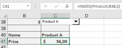
• Searching Lists:

=INDEX(PriceList; B38; 1)  // Returns product name from row B38. 

=INDEX(PriceList; B38; 2)  // Returns price from row B38. 

  Finding information  

This example demonstrates the reference version of the function. Assume that you have divided an advanced training course into three parts and offer single-unit or complete conference reservations. You also offer an early-bird discount for participants who book before a deadline. The details are shown In the figure below.

To calculate the price based on the elements booked and the reservation date, you use the following formula:

=INDEX((D47:D50;E47:E50);VLOOKUP(C53;B47:C50;2;FALSE);;IF(C54<C52

;1;2))

• Dynamic Ranges: Sum last cells of two named ranges:

=INDEX(NumberOne; ROWS(NumberOne); COLUMNS(NumberOne)) + INDEX(NumberTwo; ROWS(NumberTwo); COLUMNS(NumberTwo)) 

Notes

• Use Ctrl+Shift+Enter for array formulas (legacy Excel).
• For dynamic ranges, combine with ROWS(), COLUMNS(), or OFFSET().

This function creates a clickable hyperlink to a document, webpage, or file location.

Syntax:

HYPERLINK(link_location; [friendly_name])

Arguments:

• link_location (required):
  • A text string specifying the path or URL (e.g., « C:\Files\Report.docx » or « https://example.com »).
• friendly_name (optional):
  • The display text in the cell (e.g., « Open Report »). If omitted, the link_location is shown.

Background:

• Dynamic Links: Unlike static links (Ctrl+K), this function allows formula-based links (e.g., linking to a file path stored in another cell).
• Editing: To modify the hyperlink, click and hold the cell until the cursor turns into a cross.
• Errors: Invalid paths display an error message.

Examples:

1. Web Link (Microsoft Office Online):

=HYPERLINK(http://office.microsoft.com/de-de/default.aspx »; « Internet test ») 

1. • Displays: « Internet test » (click to open the URL).
2. Local Word Document:

=HYPERLINK(« document.docx#highlight »; « Word test ») 

 

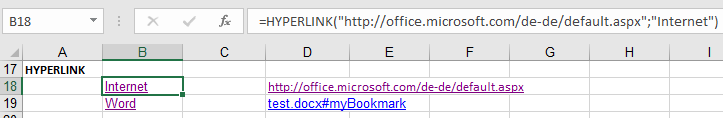
1. • Opens document.docx and jumps to the text « highlight ».
   • Displays: « Word test ».
2. Alternative Method (Copy-Paste Hyperlink):
   • In Word: Select text → Copy.
   • In Excel: Right-click → Paste as Hyperlink.

Note: Right-click the cell to edit or remove the hyperlink.

This function searches for a value in the top row of a table or array and returns a corresponding value from the specified row.

Syntax:

HLOOKUP(lookup_value; table_array; row_index_num; [range_lookup])

Arguments:

• lookup_value (optional): The value to search for (text, number, or logical value).
• table_array (required): A cell range or array constant (enclosed in braces {}).
• row_index_num (required): A positive integer indicating which row to return (must not exceed the table’s rows).
• range_lookup (optional):
  • FALSE → Searches for an exact match.
  • TRUE or omitted → Finds the nearest match (≤ lookup_value).

Background:

1. Exact Match (range_lookup = FALSE):
   • Searches the top row for an exact match of lookup_value.
   • Returns #N/A if no match is found.
   • No sorting required.
2. Approximate Match (range_lookup = TRUE or omitted):
   • Returns an exact match if found; otherwise, the largest value ≤ lookup_value.
   • Requires the top row to be sorted in ascending order.

Example:

A bus timetable requires finding minutes based on a stop (column) and time (row) as seen in the table below.

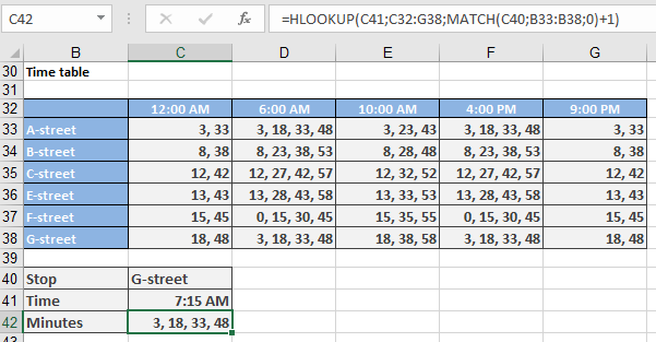
Since HLOOKUP() alone cannot handle row selection dynamically, combine it with MATCH():

=HLOOKUP(C41; C32:G38; MATCH(C40; B33:B38; 0) + 1) 

• MATCH(C40; B33:B38; 0): Finds the stop (C40) in the first column.
• +1: Adjusts for the header row in table_array.