Votre panier est actuellement vide !
Étiquette : statistical
How to use the SKEW() function in Excel
The SKEW() function returns the skewness of a distribution. Skewness measures the degree of asymmetry of a distribution around its mean.
- A positive skewness indicates a distribution with a tail that extends toward more positive values.
This is also referred to as a left-skewed distribution. - A negative skewness indicates a distribution with a tail that extends toward more negative values.
This is also called a right-skewed distribution.
Syntax:
SKEW(number1; [number2]; …)
Arguments
- number1 (required), number2 (optional):
At least one, and up to 255 arguments, representing the sample data.
You can input values individually, or use an array or cell reference.
Background
The SKEW() function calculates the skewness of a unimodal frequency distribution, focusing on how symmetric (or not) the data is around the mean.
Skewness is highly sensitive to outliers and extreme values.
In a normal (Gaussian) distribution, the skewness is 0, and the distribution is perfectly symmetrical about the mean.
In contrast:
- In a positively skewed distribution, the mean > median > mode
- In a negatively skewed distribution, the mean < median < mode
For a normal distribution:
- ~66% of data lies between the mean ± standard deviation
- The inflection points are at μ − σ and μ + σ
Formula
Skewness is defined as:
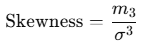
Where:
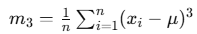 is the third central moment
- σ is the standard deviation
- μ is the mean of the distribution
Interpretation:
- If Skewness > 0, the distribution is right-skewed
- If Skewness < 0, the distribution is left-skewed
Example
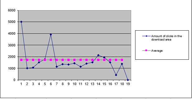
A software company wants to analyze the click behavior on their website and its download area.
The marketing team uses the SKEW() function to evaluate the asymmetry in the number of clicks for:
- The download area
- The entire website
Results:
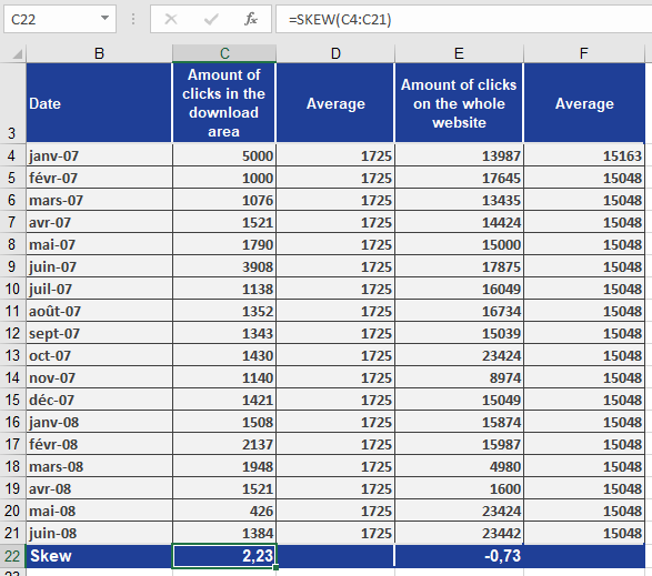
- Download area has a skewness of 2.23 → positively skewed
- This indicates the data is pulled toward higher values
- Also called left modal because the peak is on the left side of the chart
- See Figure below
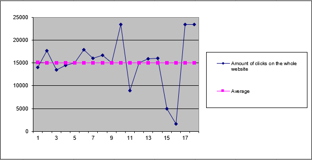
- Entire website has a skewness of -0.73 → negatively skewed
- This indicates the data is pulled toward lower values
- Also called right modal because the peak is on the right side of the chart
- See Figure below
Conclusion
The SKEW() function helps:
- Analyze distribution shape
- Detect asymmetry caused by outliers
- Compare actual data to a normal distribution
- A positive skewness indicates a distribution with a tail that extends toward more positive values.
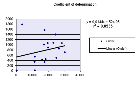
How to use the RSQ() function in Excel
This function returns the square of the Pearson correlation coefficient (r²) based on paired data points (known_y’s and known_x’s). The r² value represents the proportion of variance in the dependent variable (y) that can be explained by the independent variable (x).
Syntax:
RSQ(known_y’s; known_x’s)Arguments:
- known_y’s (required): An array or range of dependent data points (y-values)
- known_x’s (required): An array or range of independent data points (x-values)
Background:
RSQ() calculates the coefficient of determination (r²), which is the square of the Pearson correlation coefficient (r). This value indicates the strength of the linear relationship between two variables.The coefficient of determination ranges between 0 and 1, where:
- 0 indicates no linear relationship
- 1 indicates a perfect linear relationship
The Pearson correlation coefficient (r) is calculated as:
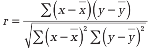
Where:
- x̄ and ȳ are the sample means (AVERAGE(x_values) and AVERAGE(y_values))
- RSQ() returns r² (r squared)
Important Notes:
- An r² value of 0.0354 suggests only 3.5% of the variation in y is explained by x
- While r² = 1 indicates a perfect linear fit, this does not imply causation
- Negative r² values are not possible and likely indicate an input error
Example:
A software company analyzes the relationship between website visits (x) and online orders (y):- Data is collected for both variables
- RSQ() calculation returns r² = 0.0535 (5.35%)
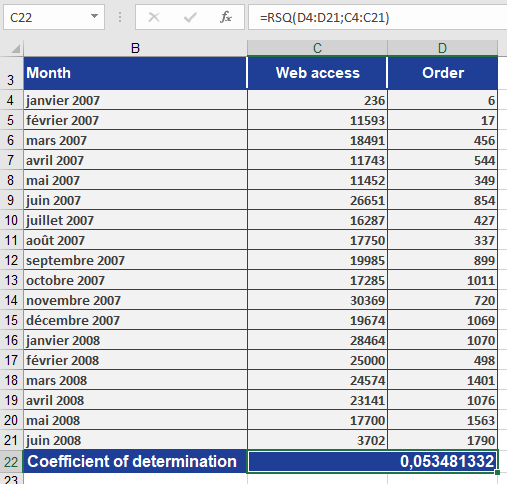
- Interpretation:
- Only 5.35% of order variation is explained by visit frequency
- This weak relationship is visually confirmed in Figure below
How to use the RANK.EQ() function in Excel
This function returns the rank of a number within a list of numbers. The rank indicates the number’s relative size compared to other values in the list. If the list were sorted, the rank would correspond to the number’s position.
Syntax:
RANK.EQ(number; ref; [order])Arguments:
- number(required): The value for which you want to determine the rank.
- ref(required): An array or reference to a list of numeric values. Non-numeric values in the reference are ignored.
- order(required): Specifies the ranking order:
- If 0or omitted: Ranks numbers as if the reference were sorted in descending order (highest value = rank 1).
- If non-zero: Ranks numbers as if the reference were sorted in ascending order (lowest value = rank 1).
Background:
For additional details about ranking functionality, refer to the documentation for the RANK() function.Example:
Usage examples for the RANK.EQ() function can be found in the figure below.
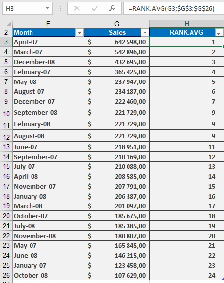
How to use the RANK.AVG() function in Excel
Returns the rank of a specified number within a dataset, using average ranking for tied values. Unlike RANK() which skips subsequent ranks for duplicates, this function assigns the average rank to all identical values.
Syntax:
RANK.AVG(number; ref; [order])Arguments
Argument Description number (required) The numeric value to be ranked. ref (required) The array or range containing the dataset. Non-numeric values are ignored. order (optional) Ranking order: - 0 (or omitted): Descending (highest value = rank 1).
- Non-zero: Ascending (lowest value = rank 1). |
Key Features
- Handling Ties:
- If multiple values are identical, they receive the average of their potential ranks.
- Example: Values (10, 20, 20, 30) ranked in descending order:
- 30 → Rank 1
- Both 20s → Average of ranks 2 and 3 → 2.5
- 10 → Rank 4
- Comparison with Other Rank Functions:
Function Behavior with Ties RANK() / RANK.EQ() Assigns same rank, skips subsequent ranks. RANK.AVG() Assigns average rank to tied values. - Use Cases:
- Fair ranking in competitions with tied scores.
- Statistical analysis requiring precise percentile calculations.
Example & Background
For practical applications (e.g., sales data ranking), see the figure below, which includes:
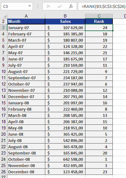
How to use the RANK() function in Excel
Returns the rank of a specified number within a dataset, indicating its relative size compared to other values. The rank represents the number’s position if the dataset were sorted.
Syntax:
RANK(number; ref; [order])Arguments
Argument Description number (required) The value to rank. ref (required) The dataset (array or range) containing numbers to compare against. Non-numeric values are ignored. order (optional) Controls ranking direction: - 0 (or omitted): Descending order (highest value = rank 1).
- Non-zero: Ascending order (lowest value = rank 1).
Key Features
- Tied Values:
- Duplicate numbers receive the same rank.
- Subsequent ranks are skipped (e.g., two values tied for rank 3 will omit rank 4).
- Correction for Ties:
To adjust ranks for identical values, use this formula:
text
[COUNT(ref) + 1 – RANK(number, ref, 0) – RANK(number, ref, 1)] / 2
Applies to both ascending and descending rankings.
- Efficiency:
Ideal for large datasets where manual ranking is impractical.
Example: Sales Performance Ranking
Scenario: A software company analyzes monthly sales over two years (24 months).
Steps:
- Data: Column A lists sales figures for each month.
- Ranking:
- Use =RANK(A2, $A$2:$A$25, 0) to rank sales in descending order (highest sale = rank 1).
- If sales are unique, ranks span 1–24 without gaps.
Result:
- Column B displays each month’s rank (see Figure below).
- Tied sales would share a rank.
Practical Notes
- Alternatives: Modern Excel versions use RANK.EQ() (identical to RANK()) and RANK.AVG() (assigns average rank to ties).
- Visualization: Combine with conditional formatting to highlight top/bottom performers.
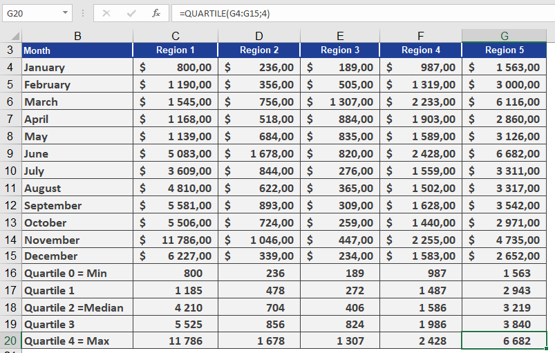
How to use the QUARTILE() function in Excel
Returns the specified quartile of a dataset. Quartiles divide data into four equal groups, useful for analyzing income distributions, sales performance, or survey results (e.g., identifying the top 25% of values).
Syntax:
QUARTILE(array ; quart)Arguments
Argument Description array (required) Range of numeric values to analyze. quart (required) Integer (0–4) specifying which quartile to return. Table 1: Quartile Argument Values
Value Result 0 Minimum value 1 25th percentile (lower quartile) 2 50th percentile (median) 3 75th percentile (upper quartile) 4 Maximum value Key Concepts
- Quartiles split data into 4 equal parts, while quantiles divide it into *n* parts.
- Median (quart=2) divides data into two equal halves.
- For datasets with even observations (e.g., 12 values), the median averages the middle two values.
Pharmaceutical Sales Example
Goal: Analyze pill sales across 5 U.S. regions per 100,000 residents.
Data: 12 monthly sales values per region (sorted in ascending order).
Calculations for Region 1:
- Quartile 0 (Min): $800
- Quartile 2 (Median):
- Position: Between 5th/6th values → (4,200 + 4,220)/2 = $4,210
- Quartile 4 (Max): $11,786
Quartiles 1 & 3 (25th/75th Percentiles):
- Quartile 1 (25%): Between 3rd/4th values → $1,185
- Interpretation: 25% of sales ≤ $1,185.
- Quartile 3 (75%): Between 9th/10th values → $5,525
- Interpretation: 75% of sales ≤ $5,525.
Comparative Insight:
- In Region 5, 75% of sales are ≤ $3,840 (vs. $5,525 in Region 1).
Manual Calculation Notes
- For n=12:
- 25th percentile: 0.25×12 = 3rd/4th values → Weighted toward 4th.
- 75th percentile: 0.75×12 = 9th/10th values → Weighted toward 10th.
Visual Reference: See Figure below for sales data.
How to use the PROB() function in Excel
This function calculates the probability of values falling within a specified range. If no upper limit is provided, it returns the probability of values equaling the lower limit exactly.
Syntax:
PROB(x_range; prob_range; lower_limit; [upper_limit])Arguments:
- x_range(required): The set of possible numerical outcomes.
- prob_range(required): The corresponding probabilities for each value in x_range (must sum to 1).
- lower_limit(required): The minimum value of the target range.
- upper_limit(optional): The maximum value of the target range.
Key Requirements:
- All probabilities must be ≥0 and ≤1.
- The sum of all probabilities must equal 1.
Background:
The PROB() function aggregates probabilities for discrete outcomes. It’s particularly useful when:- Working with known probability distributions
- Analyzing scenarios with defined outcome likelihoods
- Calculating cumulative probabilities for value ranges
Medical Example:
A doctor analyzes patient weight probabilities based on historical data:*Data Setup (Figure below)*:
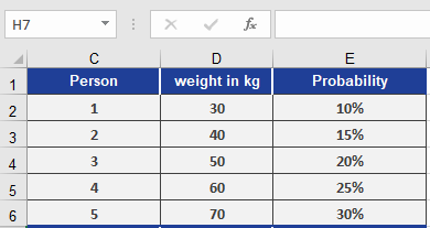
- Weights (x_range): [100, 110, 120, 140, 150] lbs
- Probabilities (prob_range): [0.1, 0.15, 0.25, 0.3, 0.2]
Calculations (Figure below):
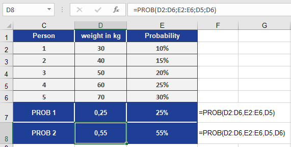
- Exact weight probability:
- =PROB(weights, probs, 120)→ 25%
(Probability of weighing exactly 120 lbs)
- =PROB(weights, probs, 120)→ 25%
- Weight range probability:
- =PROB(weights, probs, 120, 140)→ 55%
(Probability of weighing between 120-140 lbs)
- =PROB(weights, probs, 120, 140)→ 55%
Key Notes:
- When upper_limit is omitted, PROB() treats lower_limit as both min and max.
- The function sums probabilities for all x_values within the specified bounds.
How to use the POISSON.DIST() function in Excel
This function calculates probabilities for a Poisson-distributed random variable. The Poisson distribution is commonly used to predict the frequency of rare, independent events over a specific interval (e.g., call center arrivals per hour or tire failures per 100,000 miles).
Syntax:
POISSON.DIST(x ; mean ; cumulative)Arguments:
- x (required): The number of events to evaluate.
- mean (required): The expected average number of events (λ).
- cumulative (required): A logical value determining the calculation type:
- TRUE: Returns the cumulative probability (0 to *x* events).
- FALSE: Returns the exact probability for exactly *x* events.
Background:
Named after Siméon Denis Poisson (1781–1840), this distribution models rare events in large populations where:- Events are independent (e.g., radioactive decay, customer arrivals).
- The average event rate (mean) is known but the actual occurrences are sporadic.
- The probability of an event is proportional to the interval length.
Key Properties:
- Approximates the binomial distribution for low-probability, high-sample scenarios.
- Requires only the mean (λ) as a parameter (unlike the binomial distribution).
- Assumes events are:
- Rare within the interval.
- Random and independent of prior events.
Formulas:
- Exact probability (cumulative = FALSE):
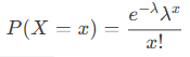
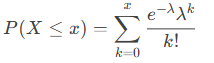
- Cumulative probability (cumulative = TRUE):
Example:
Scenario: A tire dealer observes an average of 4 damage incidents per 100,000 miles.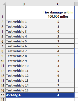
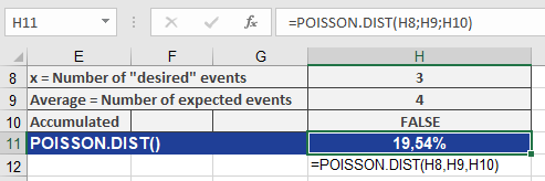
- Question: What is the probability of exactly 3 incidents?
- Inputs:
- x = 3, mean = 4, cumulative = FALSE
- Result: 19.54% (see Figure below).
- Inputs:
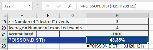
- Question: What is the probability of 0 to 3 incidents?
- Inputs:
- x = 3, mean = 4, cumulative = TRUE
- Result: 43.35% (see Figure below).
- Inputs:
How to use the PERMUT() function in Excel
This function returns the number of possible permutations when selecting *k* elements from a set of *n* elements. A permutation is an arrangement where the order of elements matters.
Syntax:
PERMUT(number; number_chosen)Arguments:
- number (required): The total number of elements (*n*).
- number_chosen (required): The number of elements to permute (*k*).
Background:
The PERMUT() function belongs to combinatorics, which calculates the number of ordered arrangements. Unlike COMBIN() (where order is irrelevant), PERMUT() treats different sequences as distinct.Key Differences:
- PERMUT(): Order matters (e.g., race rankings).
- Example: Calculating possible podium finishes (1st, 2nd, 3rd) in a 10-runner race.
- COMBIN(): Order irrelevant (e.g., lottery numbers).
- Analogy: Runners would protest if podium places were reordered alphabetically, but lottery numbers remain the same regardless of sequence.
Formula:
The number of permutations is calculated as: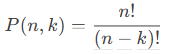
Example:
Scenario: A race with 10 runners (*n = 10*); prizes awarded for 1st, 2nd, and 3rd places (*k = 3*).
Calculation:
=PERMUT(10, 3) returns 720 possible podium arrangements.
This means there are 720 unique ways to assign gold, silver, and bronze medals among the 10 runners.Visual Reference:
See Figure below for the result.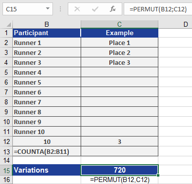
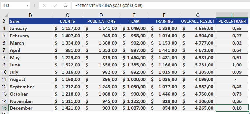
How to use the PERCENTRANK.INC() function in Excel
This function returns the rank of a value (alpha) in a dataset as a percentage, ranging from 0 to 1 (inclusive).
It can be used to evaluate the relative position of a value within a dataset. For example, you can use PERCENTRANK.INC() to assess the standing of an aptitude test score compared to all other test scores.Syntax:
PERCENTRANK.INC(array; x; [significance])Arguments:
- array(required): The array or range of numeric data that defines the relative positions.
- x(required): The value for which you want to determine the rank.
- significance(optional): A value specifying the number of decimal places for the returned percentage. If omitted, INC() defaults to three decimal places (0.xxx).
Background:
PERCENTRANK.EXC() and PERCENTRANK.INC() are the inverse functions of PERCENTILE.EXC() and PERCENTILE.INC(). These functions calculate the relative position of a value *x* within a dataset.
For additional details on quantiles, refer to the PERCENTILE() documentation.Example:
For more details on how to use this function, see the figure below