Catégorie : Excel function

The STDEVPA() function calculates the standard deviation based on an entire population, including text and logical values in the calculation.

Standard deviation measures how spread out values are from the mean. It gives insight into the consistency or variability of your dataset.

Syntax:

STDEVPA(value1; [value2]; …)

Arguments

• value1 (required), value2 (optional):
  • Up to 255 values (or 30 in Excel 2003 and earlier)
  • Can be numeric values, text, logical values, cell references, or arrays
  • Text is treated as 0
  • Logical values:
    • FALSE = 0
    • TRUE = 1

Note: To exclude text and logical values, use STDEV.P() instead.

Background

The STDEVPA() function uses the same formula as STDEV.P(), but includes logical and text values in the calculation:

Formula:

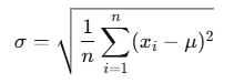
Where:

• σ = population standard deviation
• xi= each individual value (including 0 for text/FALSE, 1 for TRUE)
• μ = average (mean) of all values
• n = total number of values (including those derived from logical/text)

Example

Let’s revisit the website analysis example used for the STDEVA() function.

The software company experienced website data issues:

Month	Issue	Marked As
March 2007	Website down	« hostingproblems » (text → 0)
September 2007	Hosting problem	« hostingproblems » (text → 0)
February 2008	Access blocked	FALSE → 0
May 2008	Visits not recorded, but accessed	TRUE → 1

When applying STDEVPA() to the full set of visit data:

STDEVPA(A2:A19)

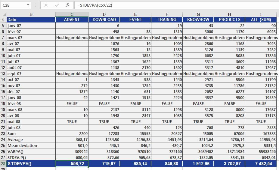
• The text and logical values are included, mapped to numeric values (as shown above).
• This leads to a different result than STDEV.P() which ignores non-numeric entries.

Result

In the PRODUCTS area:

• STDEVPA() returns 3,702.97, indicating the average deviation from the population mean, including the impact of text and logical values.

Compared to:

• STDEV.P(), which ignores these entries and thus returns a different (typically lower) value.

Conclusion

Use STDEVPA() when:

• You’re working with a complete population
• Your dataset includes text or logical values, and you want them included in your statistical analysis
• You’re handling semi-structured data, such as form responses, website logs, or datasets with missing months marked descriptively

If your data is fully numeric and clean, STDEV.P() is usually preferred.

The STDEVA() function estimates the standard deviation based on a sample. It is used to measure how dispersed or spread out values are from their mean (average).

Unlike STDEV.S(), the STDEVA() function includes text and logical values in the calculation:

• Text is treated as 0
• FALSE is treated as 0
• TRUE is treated as 1

Syntax:

STDEVA(value1; [value2]; …)

Arguments

• value1 (required), value2 (optional):
  • You can enter up to 255 arguments
  • Arguments may be numbers, text, logical values, arrays, or cell references

Note:
To exclude text and logical values from the calculation, use STDEV.S() instead.

Background

Both STDEVA() and STDEV.S() use the same mathematical formula for standard deviation. However, they differ in how they treat non-numeric data.

Formula:​

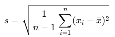
Where:

• s = sample standard deviation
• xi​ = each value in the dataset (including logic/text mapped to numeric values)
• xˉ = mean of the values
• n = number of items (including TRUE/FALSE/text as applicable)

Example

You’re analyzing monthly website visits over the past 18 months.

However, due to technical problems, the data includes:

• Text values (« hostingproblems ») for March and September 2007 (site was down)
• FALSE for February 2008 (site not accessible externally)
• TRUE for May 2008 (site accessed, but visits not recorded)

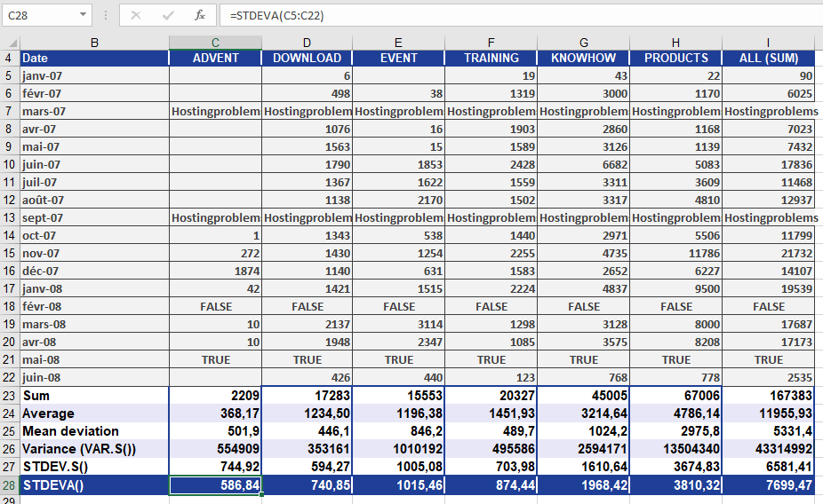
Figure below shows how this dataset looks.

Using STDEVA():

STDEVA(A2:A19)

The function includes:

• « hostingproblems » → 0
• FALSE → 0
• TRUE → 1

These values impact the mean and thus the standard deviation.

Result

In the PRODUCTS area:

• STDEVA() returns a result of 3,810.32, which means the data deviates from the mean by about 3,810.32 clicks.
• This is slightly higher than the result from STDEV.S(), because STDEVA() includes more « values » (text/logical), which reduce the mean and increase the spread.

Conclusion

Use STDEVA() when:

• Your dataset contains text or logical values
• You want those values to contribute to your statistical analysis
• You’re working with imperfect or semi-structured data (like logs, survey forms, or partial metrics)

If your dataset is strictly numeric, or you want to ignore non-numeric data, use STDEV.S() instead

The STDEV.P() function calculates the standard deviation based on an entire population. The standard deviation is a statistical measure that quantifies how much values in a dataset deviate from the mean (average).

A low standard deviation indicates that values are close to the mean, while a high standard deviation suggests that values are spread out over a wide range.

Syntax:

STDEV.P(number1; [number2]; …)

Arguments

• number1 (required), number2 (optional):
  Up to 255 numeric arguments  representing the entire population.
  You can input:
  • Individual values
  • A cell range
  • An array

 Note:

• Text and logical values (e.g. TRUE, FALSE) are ignored.
• To include text and logical values, use the STDEVA.P() function instead.

Background

The only difference between STDEV.P() and STDEV.S() is the type of data they assume:

• **STDEV.P()** assumes you are working with the entire population
• **STDEV.S()** assumes you are working with a sample of the population

Thus, they use slightly different formulas.

Formula

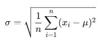
The formula used by STDEV.P() is:

Where:

• σ = population standard deviation
• xi​ = each individual value
• μ = population mean (calculated using AVERAGE(number1, …))
• n = number of data points

This formula calculates the square root of the average squared deviations from the mean.

Example

Let’s return to the website evaluation by the software manufacturer (see Figure below).

You analyze the number of clicks in the PRODUCTS area over a time period and use the STDEV.P() function to measure how much the click data varies around the average.

• The result: 3,682.85

This means that the click counts typically deviate by about 3,682.85 from the average value.

If you square this result:

(3,682.85)2=Variance=VAR.P()

Thus, you can say:

• STDEV.P() gives you the standard deviation
• VAR.P() gives you the variance, which is the square of the standard deviation

Conclusion

Use STDEV.P() when:

• You are analyzing a complete population
• You want to understand the dispersion or variability of values
• You are comparing actual vs. expected behavior, such as in web analytics, manufacturing, or financial data

The STANDARDIZE() function returns the standardized value (also called the z-score) of a data point from a distribution defined by a known mean and standard deviation.

A standardized value represents how far and in what direction a given value deviates from the mean, expressed in units of standard deviation.

Syntax:

STANDARDIZE(x; mean; standard_dev)

Arguments

• x (required): The data point you want to standardize
• mean (required): The arithmetic mean (average) of the distribution
• standard_dev (required): The standard deviation of the distribution

Background

In statistics, standardization transforms values from different scales into a common scale, typically with:

• Mean μ=0
• Standard deviation σ=1

This allows direct comparison between values from different distributions or datasets. The result is a standard normal distribution, a special case of the normal distribution where all values are expressed as z-scores.

This is based on the central limit theorem, which states that the sum of many independent, identically distributed random variables tends toward a normal distribution as the sample size increases.

Formula

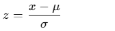
The formula used by the STANDARDIZE() function is:

Where:

• x = observed value
• μ = mean of the distribution
• σ= standard deviation of the distribution
• z = standardized (z-score) value

Example

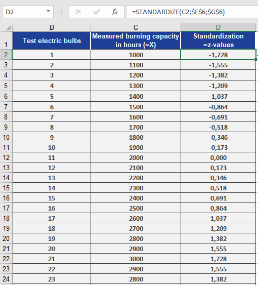
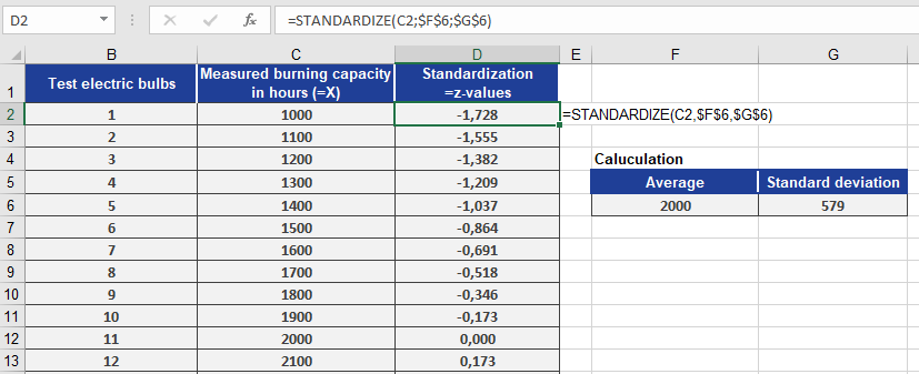
You’re a light bulb manufacturer analyzing the performance of your products. You’ve entered the measured lifespan values into an Excel table (Figure below).

You’ve also calculated:

• Mean lifespan = 2,000 hours (mean = 2000) — cell F6
• Standard deviation = 579 hours (standard_dev = 579) — cell G6

Now, you want to standardize each measured value using:

STANDARDIZE(x, 2000, 579)

Where x refers to each measured bulb’s lifespan.

Figure below shows the resulting standardized values.

Conclusion

Using the STANDARDIZE() function, you can:

• Convert raw data into z-scores
• Identify how extreme or typical a value is
• Compare values from different distributions
• Prepare data for further statistical analysis like regression, clustering, or hypothesis testing

This function is especially useful in quality control, performance benchmarking, and data normalization tasks.

Returns the k-th smallest value in a dataset. This function is useful for extracting values with specific relative rankings without sorting the data.

Syntax:
SMALL(array; k)

Arguments:

• array(required): The range or array containing the dataset
• k(required): The ordinal position of the value to return (1 = smallest, n = largest)

Key Notes:

1. Error Conditions:
   • Returns #NUM!if:
     • The array is empty
     • k ≤ 0
     • k exceeds the number of data points

2. Special Cases:
   • SMALL(array, 1)returns the minimum value
   • SMALL(array, n)(where n = count of values) returns the maximum value
3. Counterpart: This function complements LARGE()

Example – Football Attendance Analysis:
A league analyzes game attendance data:

• Dataset: Unsorted list of daily spectator counts
• Objective: Find days with lowest attendance
• Solution:
  • =SMALL(B2:B31, 1)→ Absolute minimum
  • =SMALL(B2:B31, 5)→ 5th smallest attendance

Result:
Figure below demonstrates the function returning: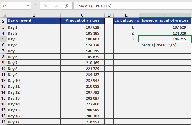

• 1st smallest value (smallest attendance day)
• 2nd smallest value

The SLOPE() function returns the slope of the linear regression line that best fits the data points in the arrays known_y’s and known_x’s.

The slope represents the rate of change — that is, the vertical change divided by the horizontal change between two points on the regression line.

Syntax:

SLOPE(known_y’s; known_x’s)

Arguments

• known_y’s (required): An array or cell range of dependent (response) variable values.
• known_x’s (required): An array or range of independent (predictor) variable values.

Background

The slope is a fundamental component in linear regression analysis. It helps determine how a change in the independent variable (x) influences the dependent variable (y).

A linear function has the general form:

yi=a+bxi

Where:

• a = y-intercept (the point where the line crosses the y-axis)
• b = slope of the line
• xi​ = individual x-values
• yi​ = corresponding y-values
• i=1,2,…,n

If both the intercept aaa and slope bbb are known, the function is fully defined. For example:

yi=2+0.4xi

In this case:

• The intercept is 2
• The slope is 0.4
• The line increases by 0.4 y-units for every increase of 1 x-unit

Formula

The slope of the regression line is calculated using the following formula:

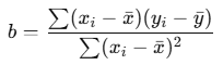
Where:

• xˉ=AVERAGE(x)
• yˉ=AVERAGE(y)

This is the formula used internally by the SLOPE() function.

Example

You are the marketing manager at a software company. You want to analyze how the number of website visits affects the number of online orders over the past 18 months.

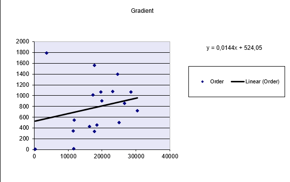
After collecting the data, you apply the SLOPE() function to the visits and orders:

SLOPE(orders_range ; visits_range)

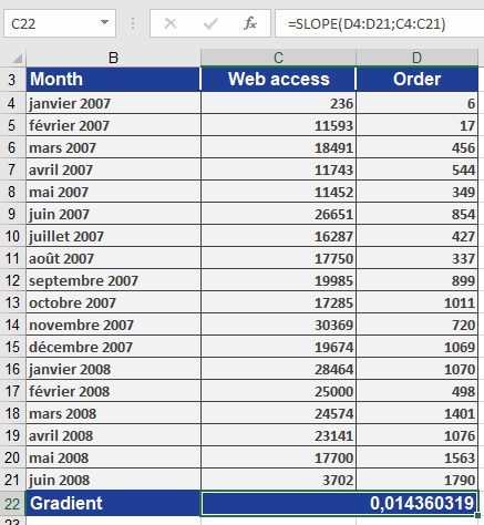
The result:

slope=0.0144\text{slope} = 0.0144slope=0.0144

This means:

• For each additional website visit, the number of orders increases by 0.0144
• In practical terms, if website visits increase by 100, the number of orders would increase by:

100×0.0144=1.44 orders100 

The  Figure below displays the regression line visually.

Conclusion

Use the SLOPE() function to:

• Calculate the rate of change between two variables
• Identify trends and relationships in data
• Create forecast models in combination with INTERCEPT(), FORECAST(), or LINEST()

The SKEW() function returns the skewness of a distribution. Skewness measures the degree of asymmetry of a distribution around its mean.

• A positive skewness indicates a distribution with a tail that extends toward more positive values.
  This is also referred to as a left-skewed distribution.
• A negative skewness indicates a distribution with a tail that extends toward more negative values.
  This is also called a right-skewed distribution.

Syntax:

SKEW(number1; [number2]; …)

Arguments

• number1 (required), number2 (optional):
  At least one, and up to 255 arguments, representing the sample data.
  You can input values individually, or use an array or cell reference.

Background

The SKEW() function calculates the skewness of a unimodal frequency distribution, focusing on how symmetric (or not) the data is around the mean.

Skewness is highly sensitive to outliers and extreme values.

In a normal (Gaussian) distribution, the skewness is 0, and the distribution is perfectly symmetrical about the mean.

In contrast:

• In a positively skewed distribution, the mean > median > mode
• In a negatively skewed distribution, the mean < median < mode

For a normal distribution:

• ~66% of data lies between the mean ± standard deviation
• The inflection points are at μ − σ and μ + σ

Formula

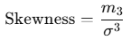
Skewness is defined as:

Where:

•   is the third central moment
• σ is the standard deviation
• μ is the mean of the distribution

Interpretation:

• If Skewness > 0, the distribution is right-skewed
• If Skewness < 0, the distribution is left-skewed

Example

A software company wants to analyze the click behavior on their website and its download area.

The marketing team uses the SKEW() function to evaluate the asymmetry in the number of clicks for:

1. The download area
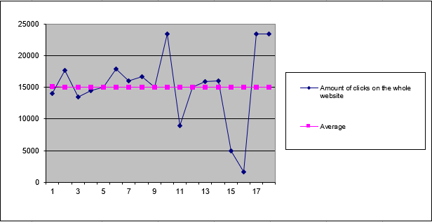
2. The entire website

Results:

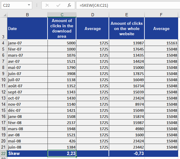
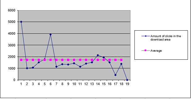
• Download area has a skewness of 2.23 → positively skewed
  • This indicates the data is pulled toward higher values
  • Also called left modal because the peak is on the left side of the chart
  • See Figure below

• Entire website has a skewness of -0.73 → negatively skewed
  • This indicates the data is pulled toward lower values
  • Also called right modal because the peak is on the right side of the chart
  • See Figure below

Conclusion

The SKEW() function helps:

• Analyze distribution shape
• Detect asymmetry caused by outliers
• Compare actual data to a normal distribution

This function returns the square of the Pearson correlation coefficient (r²) based on paired data points (known_y’s and known_x’s). The r² value represents the proportion of variance in the dependent variable (y) that can be explained by the independent variable (x).

Syntax:
RSQ(known_y’s; known_x’s)

Arguments:

• known_y’s (required): An array or range of dependent data points (y-values)
• known_x’s (required): An array or range of independent data points (x-values)

Background:
RSQ() calculates the coefficient of determination (r²), which is the square of the Pearson correlation coefficient (r). This value indicates the strength of the linear relationship between two variables.

The coefficient of determination ranges between 0 and 1, where:

• 0 indicates no linear relationship
• 1 indicates a perfect linear relationship

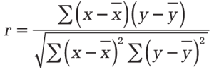
The Pearson correlation coefficient (r) is calculated as:

Where:

• x̄ and ȳ are the sample means (AVERAGE(x_values) and AVERAGE(y_values))
• RSQ() returns r² (r squared)

Important Notes:

1. An r² value of 0.0354 suggests only 3.5% of the variation in y is explained by x
2. While r² = 1 indicates a perfect linear fit, this does not imply causation
3. Negative r² values are not possible and likely indicate an input error

Example:
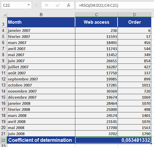
A software company analyzes the relationship between website visits (x) and online orders (y):

1. Data is collected for both variables
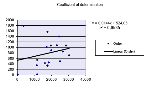
2. RSQ() calculation returns r² = 0.0535 (5.35%)

1. Interpretation:
   • Only 5.35% of order variation is explained by visit frequency
   • This weak relationship is visually confirmed in Figure below

This function returns the rank of a number within a list of numbers. The rank indicates the number’s relative size compared to other values in the list. If the list were sorted, the rank would correspond to the number’s position.

Syntax:
RANK.EQ(number; ref; [order])

Arguments:

• number(required): The value for which you want to determine the rank.
• ref(required): An array or reference to a list of numeric values. Non-numeric values in the reference are ignored.
• order(required): Specifies the ranking order:
  • If 0or omitted: Ranks numbers as if the reference were sorted in descending order (highest value = rank 1).
  • If non-zero: Ranks numbers as if the reference were sorted in ascending order (lowest value = rank 1).

Background:
For additional details about ranking functionality, refer to the documentation for the RANK() function.

Example:
Usage examples for the RANK.EQ() function can be found in the figure below.

Returns the rank of a specified number within a dataset, using average ranking for tied values. Unlike RANK() which skips subsequent ranks for duplicates, this function assigns the average rank to all identical values.

Syntax:
RANK.AVG(number; ref; [order])

Arguments

Argument	Description
number (required)	The numeric value to be ranked.
ref (required)	The array or range containing the dataset. Non-numeric values are ignored.
order (optional)	Ranking order:

• 0 (or omitted): Descending (highest value = rank 1).
• Non-zero: Ascending (lowest value = rank 1). |

Key Features

1. Handling Ties:
   • If multiple values are identical, they receive the average of their potential ranks.
   • Example: Values (10, 20, 20, 30) ranked in descending order:
     • 30 → Rank 1
     • Both 20s → Average of ranks 2 and 3 → 2.5
     • 10 → Rank 4
2. Comparison with Other Rank Functions:

Function	Behavior with Ties
RANK() / RANK.EQ()	Assigns same rank, skips subsequent ranks.
RANK.AVG()	Assigns average rank to tied values.

1. Use Cases:
   • Fair ranking in competitions with tied scores.
   • Statistical analysis requiring precise percentile calculations.

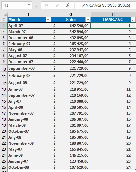
Example & Background

For practical applications (e.g., sales data ranking), see the figure below, which includes: