Catégorie : Excel function

The F.INV.RT() function returns the inverse of the right-tailed F-distribution. If p = F.DIST.RT(x,…), then F.INV.RT(p,…) = x.

The F-distribution is used in an F-test to compare variances between two data sets. For example, you could analyze income distributions in the United States and Canada to determine whether the two countries exhibit similar income diversity.

Syntax

F.INV.RT(probability; degrees_freedom1; degrees_freedom2)

Arguments

• probability (required): The probability associated with the F-distribution (e.g., significance level α).
• degrees_freedom1 (required): The degrees of freedom in the numerator.
• degrees_freedom2 (required): The degrees of freedom in the denominator.

Background

• The output of an ANOVA (Analysis of Variance) often includes:
  • The F-statistic
  • The F-probability (p-value)
  • The critical F-value at a specified significance level (e.g., 0.05).
• This function helps test whether the means of two or more samples are statistically equal.
• It evaluates if observed differences in group means are significant or due to random variation.

The F.INV.RT() function calculates the critical F-value for a given significance level (α). By comparing this critical value to the calculated F-statistic, you can accept or reject the null hypothesis.

Example

Scenario:
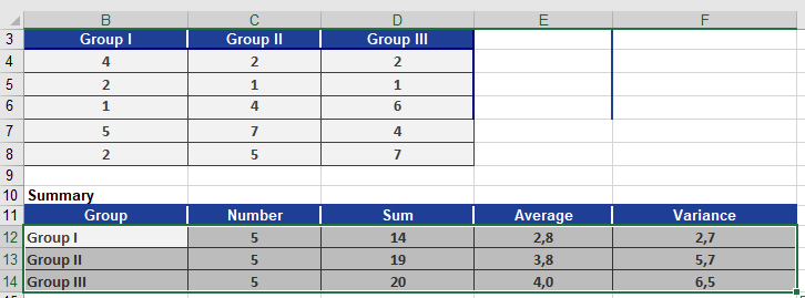
You are an occupational therapist studying how strongly employees identify with their company.

• Sample: 15 employees, each answering 10 questions (with 3 answer options per question).
• Data is summarized (Figure below).

Hypotheses:

• Null hypothesis (H₀): No difference exists between the three employee groups.
• Alternative hypothesis (H₁): A significant difference exists.
• Significance level (α): 0.05 (5%).

ANOVA Results (Figure below):

• Between-group variance: Measures differences across groups.
• Within-group variance: Measures random differences among individuals in the same group.

Degrees of Freedom:

• df1 (within groups): (5–1) + (5–1) + (5–1) = 12
• df2 (between groups): 3 groups – 1 = 2

Key Calculations:

1. F-statistic: 0.42 (cell F19).
2. Critical F-value: Calculated via F.INV.RT(0.05, 2, 12).

Conclusion:

• If the F-statistic ≥ Critical F-value, reject H₀.
• Here, 0.42 < Critical Value → H₀ is accepted.
• Interpretation: No significant difference exists between the groups.

Key Notes

• F.INV.RT() computes the threshold F-value for a given α.
• Compare this critical value to your F-statistic to decide on H₀.
• Retain H₀ if F-statistic < Critical Value (no significant difference).

This function returns the values of a distribution function (1 – alpha) of a right-tailed F-distributed random variable. Use this function to determine whether two data sets have different variances.

For example, you can compare the survey results of three equal employee groups to determine whether the variance in results is statistically different.

Syntax

F.DIST.RT(x; degrees_freedom1; degrees_freedom2)

Arguments

• x (required): The value at which to evaluate the function.
• degrees_freedom1 (required): The degrees of freedom in the numerator.
• degrees_freedom2 (required): The degrees of freedom in the denominator.

Background

• The F.DIST.RT() function returns the significance level (probability) based on a given F-value.
• It calculates the probability (significance level) for the critical F-values determined by F.INV.RT().
• The F.INV.RT() function, in contrast, calculates the critical F-value based on a given probability and degrees of freedom.

Example

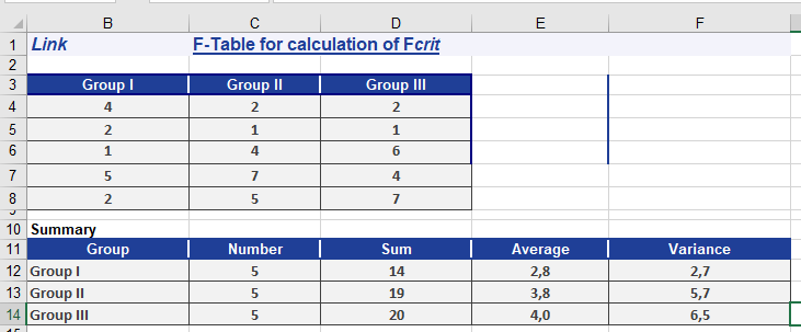
In a survey, 15 employees answered 10 questions, each with three possible answers (see Figure below).

• Null hypothesis (H₀): No difference exists between the three groups.
• Alternative hypothesis (H₁): A significant difference exists.

A variance analysis returns the results shown in Figure below.

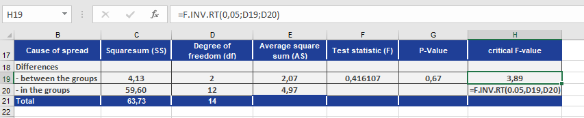
• Using F.INV.RT() with a significance level (α) of 0.05, the critical F-value is calculated as 3.89.
• F.DIST.RT() returns a significance level of 0.05 for this critical value.

The function uses the values from Figure  to compute F.DIST.RT().

The calculation of the significance level for F produces the result shown in Figure below.

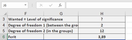
• F.DIST.RT() returns a probability of 0.67 (67%) for the test statistic F = 0.4161 (see Figure below).

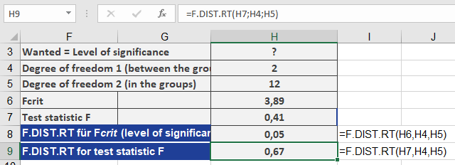
Since the significance level (α = 0.05) is less than the p-value (0.67), the null hypothesis is not rejected. This means there is no significant difference between the groups.

Key Notes

• F.DIST.RT() calculates the right-tailed probability (significance level) for a given F-statistic.
• If the returned p-value > α, the null hypothesis is retained (no significant difference).
• If p-value ≤ α, the null hypothesis is rejected (significant difference exists).

This function calculates probabilities for an exponentially distributed random variable, modeling the time between independent events. It is commonly used to predict waiting times, such as:

• The time until a call center receives the next call.
• The duration between ATM transactions.

Syntax

EXPON.DIST(x ; lambda ; cumulative)

Arguments

• x (required): The time value for which you want to calculate the probability.
• lambda (required): The rate parameter (average events per time unit).
  • Example: If calls average 3 per minute, lambda = 3.
• cumulative (required):
  • TRUE: Returns the cumulative distribution function (CDF) (probability of an event occurring by time x).
  • FALSE: Returns the probability density function (PDF) (likelihood of an event occurring at exactly time x).

Background

Key Properties

• Memoryless Process: The probability of an event occurring in the next interval is independent of past events.
• Decay/Growth: Models processes where values change by a constant factor over equal intervals (e.g., radioactive decay, call arrivals).
• Inverse: The natural logarithm is the inverse of the exponential function (base *e*, Euler’s number ≈ 2.71828).

Formulas

1. Probability Density Function (PDF):

f(x;λ)=λe−λx(Likelihood at exact time x)

1. Cumulative Distribution Function (CDF):

F(x;λ)=1−e−λx(Probability of event occurring by time x)

Example

Let’s use with the example of the call center. Assume that you operate a call center for a printer manufacturer. The call center is open 24 hours a day, seven days a week. You want to analyze the call pattern and count the incoming calls every hour over one day. This means that the time interval is 60 minutes.

The recorded calls result in the statistics shown in Figure below.

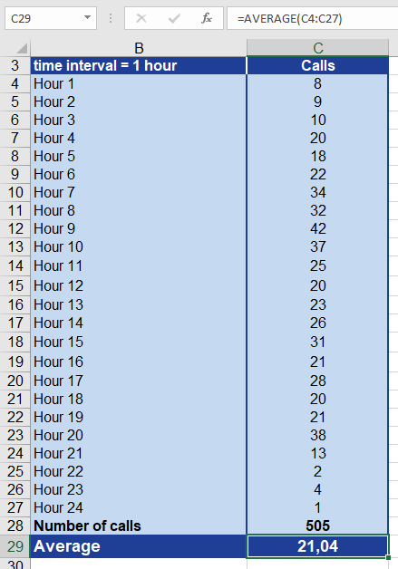
After you have calculated the average of all incoming calls, you can make the following statements:

Every hour, an average of 21 calls come in.

This means that, on average, every three minutes a customer calls.

Now you want to know the probability that a customer will call after two minutes. To find out, you use the EXPON.DIST() function. What information do you have to enter for the arguments?

x = 2, because we want to calculate the probability for a call after 2 minutes.

Lambda = 3, because this is the mean value of events per interval and therefore the passed value.

cumulative = TRUE, because in our example the cumulative distribution should be returned.

Figure below shows the result from the calculation of the probability with the EXPON.DIST() function.

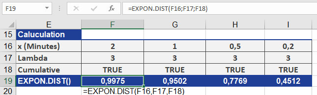
The probability for a call coming in after two minutes is 99 percent.

As you can see in figure above, the probability decreases as the time interval decreases. This means that the probability for a call to come in after

0.2 minutes (12 seconds) is only 45 percent.

Key Notes

• Lambda (λλ): Must match the time unit of x (e.g., if x is in minutes, lambda = events/minute).
• Common Uses:
  • Reliability analysis (e.g., time until failure).
  • Queueing theory (e.g., wait times).
• Visualization: Exponential distributions have a steep decay curve.

This function calculates the sum of squared deviations of data points from their sample mean. It measures the total variability (dispersion) within a dataset.

Syntax

DEVSQ(number1; [number2]; …)

Arguments

• number1 (required): The first numerical value or range.
• number2, … (optional): Additional values or ranges (up to 255 arguments in modern Excel).
• Note: You can use a single array (e.g., A2:A10) instead of comma-separated arguments.

Background

Regression & Correlation

• Correlations between variables are quantified using coefficients (e.g., Pearson’s *r*).
• Regression models predict a dependent variable (*y*) from an independent variable (*x*). A linear model assumes a straight-line relationship (e.g., « as *x* increases, *y* increases/decreases »).
• Model quality is often assessed using R² (the proportion of variance explained by the model).

Forecast Error & Variability

• The mean (average) is the simplest predictor of *y*. Deviations from the mean are called forecast errors.
• Variance (calculated with VAR.S()) averages these squared deviations.
• DEVSQ() sums these squared deviations, providing a raw measure of total variability.

Formula

Where:

• xi = Individual data points.
• xˉ = Sample mean (AVERAGE of the data).

Example

Scenario: Analyzing the relationship between website visits (*x*) and online orders (*y*).

• Goal: Calculate the total squared deviations of website visits from their mean to assess data spread.
• Result: DEVSQ () returns 1,109,624,270 (see Figure below), matching the manual sum of squared deviations.

Why Use DEVSQ()?

1. Regression Analysis: Used in calculating SST (Total Sum of Squares) for R².
2. Statistical Tests: Helps evaluate data dispersion (e.g., ANOVA).
3. Quality Control: Monitors variability in processes.

Key Notes

• Difference from VAR.S():
  • VAR.S() divides DEVSQ() by n−1 to compute sample variance.
  • DEVSQ() provides the numerator of variance formulas.
• Units: Output is in squared units of the original data (e.g., « visits² »).

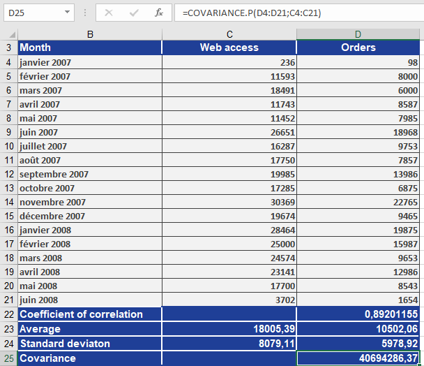
This function calculates the population covariance, which is the average of the products of deviations for each pair of data points. Covariance helps determine the relationship between two datasets. For example, you can analyze whether higher income levels correlate with higher education levels.

Syntax

COVARIANCE.P(array1; array2)

Arguments

• array1 (required): The first range of integer values.
• array2 (required): The second range of integer values.

EXAMPLE

Key Notes

• Population vs. Sample: Unlike COVARIANCE.S (sample covariance), COVARIANCE.P calculates covariance for an entire population.
• Interpretation:
  • Positive result: Indicates a direct relationship (as one variable increases, the other tends to increase).
  • Negative result: Indicates an inverse relationship (as one variable increases, the other tends to decrease).
  • Zero: Suggests no linear relationship.

This function returns the covariance of two sets of values. Covariance helps determine the relationship between two datasets. For example, you can analyze whether an increase in online orders correlates with the number of website visits. To compute covariance, the deviations of all value pairs from their respective means are multiplied, and then the average of these products is taken.

Syntax

COVAR(array1; array2)

Arguments

• array1 (required): The first range of integer values.
• array2 (required): The second range of integer values.

Background

The covariance describes the correlation between two variables, *x* and *y*, in terms of direction (positive or negative). It indicates whether the relationship between the variables is direct or inverse. Covariance can take any real value.

Interpreting Covariance Results

• Positive covariance: Indicates a concordant linear relationship between *x* and *y*. High values of *x* correspond to high values of *y*, and low values of *x* correspond to low values of *y*.
• Negative covariance: Indicates an inverse linear relationship. High values of one variable correspond to low values of the other.
• Zero covariance: Suggests no linear correlation between *x* and *y*.

While covariance reveals the direction of the relationship, it does not measure the strength of the correlation. This is because covariance depends on the scale of the variables. For instance, a covariance of 5.2 meters would be 520 centimeters for the same data in a different unit.

Key Insights from Covariance and Standard Deviations

Given *n* pairs of values (x₁, y₁), (x₂, y₂), …, (xₙ, yₙ), with standard deviations sₓ and sᵧ and covariance sₓᵧ, the maximum possible covariance is the product of the standard deviations (sₓ × sᵧ). This upper limit occurs when the relationship between xᵢ and yᵢ is linear (i.e., y = a + bx).

The covariance is calculated as:

COVAR=∑(xi−xˉ)(yi−yˉ)nCOVAR=n∑(xi​−xˉ)(yi​−yˉ​)​

where:

• x̄ and ȳ are the sample means (AVERAGE(array1) and AVERAGE(array2)).
• n is the sample size.

Example

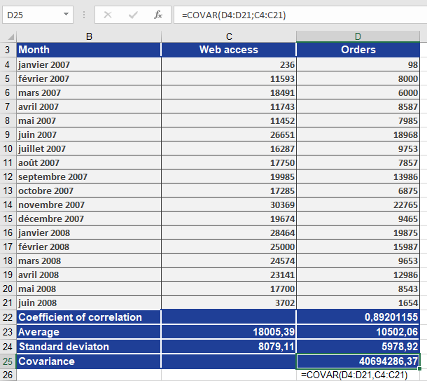
Consider a software company that sells products online and uses newsletters to boost sales. Last year, website orders increased significantly. To understand the reason, you first calculated the correlation coefficient. Now, you want to determine the direction of the relationship between website visits (*x*) and online orders (*y*) by computing the covariance.

The positive covariance confirms a concordant linear relationship—higher website visits correspond to higher orders, and lower visits correspond to fewer orders. This is further supported by a correlation coefficient of 0.89, indicating a strong linear relationship.

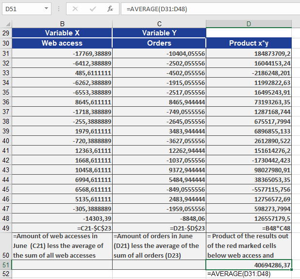
A manual calculation (without COVAR()) using the formula above yields the same result, as illustrated in the accompanying figures.

This function counts cells that meet multiple specified conditions across different ranges. It extends COUNTIF() by supporting multiple criteria.

Syntax
COUNTIFS(criteria_range1; criteria1; [criteria_range2; criteria2]; …)

Arguments

• criteria_range1 (required): First range to evaluate
• criteria1 (required): Condition for criteria_range1 (number, expression, text, or reference)
• criteria_range2, criteria2,… (optional): Additional range/criteria pairs (up to 127 pairs)

Key Features

• All ranges must be the same size
• Only counts cells where ALL conditions are met (logical AND)
• Ignores empty cells and text in numeric ranges
• Supports same comparison operators as COUNTIF() (e.g., « >150000 »)
• Case-insensitive for text criteria
• Wildcards supported: ? (single char), * (any sequence)

Example: Yearly Sales Comparison
Using the software company’s 24-month sales data:

1. Total months >$150,000 (both years):

=COUNTIFS(C3:C26, »>150000″)

1. Year-specific analysis (2007 vs 2008):
   • For 2007:

=COUNTIFS(C3:C14, »>150000″,B3:B14,2007)

1. • For 2008:

=COUNTIFS(C15:C26, »>150000″,B15:C26,2008)

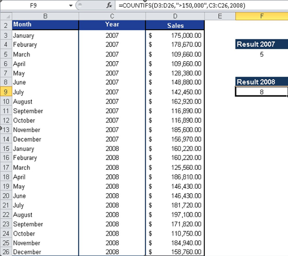
Results (Figure below):

• 2007: 7 months above target
• 2008: 15 months above target
• Improvement: 8 additional months achieved target in 2008

Practical Applications

• Multi-condition data analysis
• Year-over-year performance comparisons
• Complex filtering without pivot tables
• Data validation across multiple parameters

Note: For OR logic between criteria (counting if EITHER condition is met), use multiple COUNTIFS() functions summed together.

This function counts the number of cells within a specified range that meet a single specified condition.

Syntax
COUNTIF(range; criteria)

Arguments

• range (required): The group of cells to evaluate (can be numbers, text, or references)
• criteria (required): The condition that determines which cells to count, which can be:
  • A number (e.g., 2000)
  • Text (e.g., « Completed »)
  • A cell reference (e.g., B5)
  • A comparison expression (e.g., « >200000 »)

Background
While categorized as a statistical function, COUNTIF() serves as a powerful conditional counting tool. Note these technical requirements:

• For comparison operators (<, >, <=, >=, <>), the criteria must be enclosed in quotation marks
• The function supports wildcards: ? (single character) and * (any sequence)
• Case-insensitive for text criteria

Examples

Example 1: Sales Target Analysis
Using the software company’s 24-month sales data (range C3:C26):

=COUNTIF(C3:C26, »>200000″)

Returns: 15

Interpretation: The $200,000 monthly sales target was achieved 15 times in the 24-month period.

Special Syntax Notes

• For « less than 0 » criteria: « <0 »
• For « not empty » criteria: « <> »
• To reference another cell’s value as criteria: « <« &B1

Practical Applications

• Performance tracking against targets
• Inventory level monitoring
• Survey response categorization
• Data validation and completeness checks

This function calculates the number of empty cells within a specified range. Unlike COUNT() and COUNTA(), it specifically tallies blank cells.

Syntax
COUNTBLANK(range)

Arguments

• range(required): The cell range to evaluate for empty cells

Background
Particularly valuable for:

• Data validation and completeness checks
• Large datasets where manual counting would be impractical
• Complementing COUNT() and COUNTA() to provide complete cell analysis

Key Features

• Counts truly empty cells (no data or formulas)
• Also counts cells containing:
  • Formulas that return empty strings («  »)
  • Formulas that return NULL values
• Does not count cells with:
  • Space characters
  • Zero values
  • Text strings (even if blank-appearing)

Example
Using the same data range (C3:C25) from the COUNT() function example:
=COUNTBLANK(C3:C25)
Returns: 3

Interpretation
This indicates there are 3 completely empty cells in the range C3:C25. When combined with COUNTA() results (which returned 19 for the same data), you can verify complete data coverage:

• 19 cells with data (COUNTA)
• 3 empty cells (COUNTBLANK)
• Total of 22 cells accounted for (matches range size)

Practical Application
Useful for:

• Identifying missing data entries
• Tracking form completion status
• Validating data imports
• Monitoring data collection progress

This function counts the number of non-empty cells in an argument list. Use COUNTA() to determine how many cells in a range or array contain any type of data.

Syntax
COUNTA(value1; [value2]; …)

Arguments

• value1(required): The first item, cell reference, or range to evaluate
• value2,…(optional): Additional items to evaluate (up to 255 arguments total, or 30 in Excel)

The function counts:

• All data types (numbers, text, logical values, error values)
• Empty text strings («  »)
• Formulas that return empty strings («  »)

Excludes:

• Truly empty cells
• Cells containing formulas that return nothing

Background
Similar to COUNT(), but more inclusive:

• COUNT() only tallies numeric values
• COUNTA() counts all non-empty cells regardless of content type
• Particularly useful for mixed data types or when tracking data completeness

Example
Referring to Figure below, the function:
=COUNTA(C3:C25)
Returns 20 because:

• Counts all cells with values (numbers, text, etc.)
• Includes the word « closed » in the range
• Excludes only completely empty cells

Key Difference from COUNT()
COUNTA() provides a complete occupancy count, while COUNT() gives only numeric entries. Choose based on whether you need to:

• Count all data (COUNTA)
• Count only numbers (COUNT)