Catégorie : Excel function

This function checks whether an entry is text and returns the text value. If the entry is not a text value, the return value is empty.

Syntax:
T(value)

Arguments:

• value(required): The expression (a number, text, a formula without an equal sign, a logical value, an error value, a reference, or a name) to check.

Background:
The T() function is provided for compatibility with other spreadsheet software. You do not normally need to use the T() function in formulas, because Excel automatically converts values as needed.

When using this function, keep in mind that:

• Numbers are notconverted into numerals; instead, the result is an empty string.
• Logical values (TRUE/FALSE) also return an empty string.
• Error values remain as error values and are notconverted into text.

Example of the T() Function

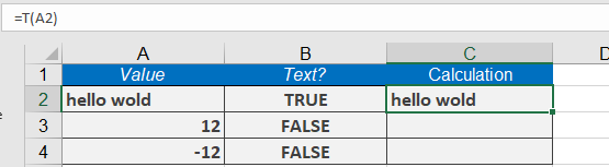
• Suppose you have the following data in cell A1:
  « Hello World »(a text string)
• Formula:
  =T(A2)
• Result:
  « Hello World »(returns the text unchanged)

The SUBSTITUTE() function replaces characters or strings with new text.

Syntax:
SUBSTITUTE(text; old_text; new_text; [instance_num])

Arguments:

• text(required): The text or the reference to a cell containing text in which you want to substitute characters.
• old text(required): The string you want to replace.
• new text(required): The string you want to replace old text
• instance Num(optional): Specifies which occurrence of old text you want to replace with new text. If you specify instance Num, only that occurrence of old text is replaced; otherwise, every instance of old text is replaced.

Background:
Use this function to replace a string of text with alternative text. The replacement can be for a single or for multiple instances.

You can use the SUBSTITUTE() function to replace a specific string within text. Use the REPLACE() function to replace a string at a certain position within text.

Example:

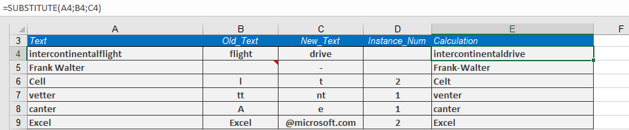
Here are some few examples:

• =SUBSTITUTE(« intercontinentalflight »; « flight »; « drive »)→ « intercontinentaldrive »
• =SUBSTITUTE(« cell » ; « l » ; « t » ; 2)→ « celt »
• =SUBSTITUTE(« vetter » ; « tt » ; « nt » ; 1)→ « venter »
• =SUBSTITUTE(« canter »; « A »; « e »)→ « canter » (no change, as « A » is not found)
• =SUBSTITUTE(« million »; « m »; « b »)→ « billion »

The SEARCH() function locates the starting position of a substring within text, beginning at start_num.
The SEARCHB() function performs the same operation for double-byte character sets (counting bytes).

Syntax
SEARCH(find_text; within_text; [start_num])
SEARCHB(find_text; within_text; [start_byte])

Key Features

• Case-insensitive (unlike FIND())
• Supports wildcards:
  • ? matches any single character
  • * matches any sequence of characters
  • Use ~ to search for literal ? or *

Arguments

Behavior Notes

• Returns #VALUE! if:
  • Text not found
  • start_num ≤ 0
  • start_num > length of within_text
• Returns 1 (or start_num) if searching for empty string («  »)

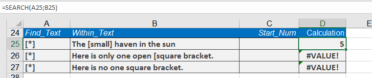
Example: Wildcard Search
To find any text in square brackets:

=SEARCH(« [*] »; « Product [small] version »)

Returns 5 (position of [small])

Comparison with FIND

Practical Applications

• Extracting substrings (combined with MID())
• Validating text patterns
• Processing structured data like codes or identifiers

The RIGHT() function extracts the specified number of characters from the end of a string.
The RIGHTB() function performs the same operation for double-byte character sets (DBCS), counting bytes instead of characters.

Syntax
RIGHT(text; num_chars)
RIGHTB(text; num_bytes)

Arguments

• text (required): The string containing characters to extract
• num_chars/num_bytes (optional):
  • Number of characters/bytes to extract (default=1 if omitted)
  • Must be ≥0

Key Features

• Returns the entire string if num_chars exceeds string length
• Part of the essential text function trio with LEFT() and MID()
• Ideal for structured data like:
  • ZIP/postal codes
  • ISBN numbers
  • Formatted identifiers

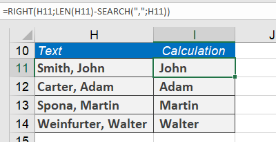
Example: Extracting Last Names
For cell H4 containing « John Smith »:

=RIGHT(H4; LEN(H4) – SEARCH( » « ; H4))

How it works:

1. SEARCH( » « ;H4) finds the space position (5)
2. LEN(H4) gets total length (10)
3. Calculation: 10 – 5 = 5 characters to extract
4. Returns « Smith »

Error Handling

• Returns #VALUE! if num_chars is negative
• Handles numbers in text by treating them as characters

This function repeats a text string a specified number of times.

Syntax
REPT(text; number_times)

Arguments

• text (required): The character or string to repeat.
• number_times (required): A positive number specifying repetition count.

Background
The REPT() function is useful for:

• Creating repeated patterns (e.g., filling cells with characters).
• Generating in-cell bar charts or visual indicators.

Key Notes:

• Returns «  » (empty string) if number_times is 0.
• Truncates decimal values (e.g., 3.9 becomes 3).
• Returns #VALUE! if:
  • number_times is negative.
  • Result exceeds 32,767 characters.

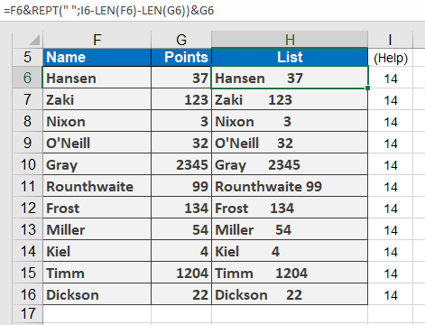
Example: Aligning Names and Scores

1. Setup:
   • Names in F6:F16, scores in G6:G16.
   • Goal: Combine in H6:H16 with aligned spacing.
2. Step 1: Calculate Max Length
   Select I6:I16 and enter (as an array formula with Ctrl+Shift+Enter):

=MAX(LEN(F6:F16) + LEN(G6:G16)) + 1

Result: Determines maximum combined length for alignment.

1. Step 2: Align Text
   In H6, enter:

=F6 & REPT( » « , I6 – LEN(F6) – LEN(G6)) & G6

How it works:

1. • Repeats spaces ( » « ) to pad between names and scores.
   • Adjusts spacing dynamically based on each row’s text length.

The REPLACE() function substitutes a portion of old_text (beginning at start_num and spanning num_chars) with new_text.
The REPLACEB() variant handles double-byte characters (using byte counts instead of character counts).

Syntax
REPLACE(old_text; start_num; num_chars; new_text)
REPLACEB(old_text; start_num; num_bytes; new_text)

Arguments

• old_text (required): The original string to modify.
• start_num (required): The position (1-based) where replacement begins.
• num_chars/num_bytes (required): The length of text to replace (in characters/bytes).
• new_text (required): The text to insert.

Background
Use REPLACE() to:

• Swap fixed-length segments within strings (e.g., placeholders or formatted sections).
• Modify specific positional patterns (unlike SUBSTITUTE(), which replaces all occurrences of a substring).

Key Differences from SUBSTITUTE

• REPLACE() targets text by position/length.
• SUBSTITUTE() replaces all instances of a specific substring.

Examples

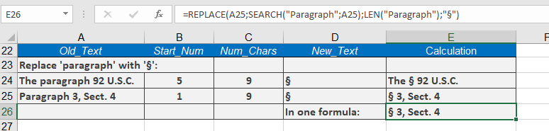
1. Replacing a word with a symbol
   Cell B25 contains « Paragraph 3, Sect. 4 »:

=REPLACE(A25; SEARCH(« paragraph »; A25); LEN(« paragraph »); « § »)

Result: « § 3, Sect. 4 »

Additional Notes

• Returns #VALUE! if start_num exceeds old_text length.
• For partial replacements (e.g., middle characters in a word), combine with LEFT(), RIGHT(), or MID().

This function converts the first character of each word in a text string to uppercase and all subsequent characters to lowercase.

Syntax
PROPER(text)

Arguments

• text(required): The text to convert, which can be:
  • A string enclosed in quotation marks
  • A formula that returns text
  • A reference to a cell containing text

Background
The PROPER() function is particularly useful for:

• Formatting imported data that is in all uppercase.
• Standardizing names or titles (including hyphenated names).
• Numeric values are treated the same as in the UPPER()

Examples

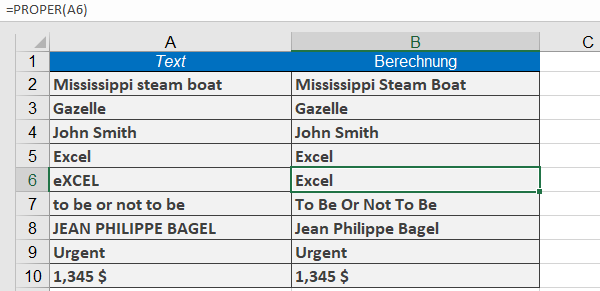
• =PROPER(« charles dickens »)returns Charles Dickens.
• =PROPER(« Excel »)returns Excel.
• =PROPER(« eXCEL »)returns Excel.
• =PROPER(« JEAN PHILIPPE BAGEL »)returns Jean Philippe Bagel.

This function extracts the phonetic (Furigana) characters from a Japanese text string.

Syntax
PHONETIC(reference)

Arguments

• reference(required): A text string or reference to a cell/cell range containing Furigana characters.
  • If referencing a range, returns Furigana from the upper-left cell.
  • Returns #N/Afor non-contiguous ranges.

Background
The Japanese writing system uses:

1. Kanji: Chinese-derived ideographs
2. Kana: Syllabic scripts including:
   • Hiragana: For native Japanese words
   • Katakana: For foreign words, loanwords, and emphasis

Furigana are small Hiragana characters that annotate Kanji pronunciation.

Notes:

• Requires Asian language support installed.
• Primarily useful for Japanese text processing.
• Most Excel users may not need this function.

The MID() function extracts characters from the middle of a text string, starting at a specified position (start_num) and returning a defined number of characters (num_chars). The MIDB() function is used for double-byte characters, where num_bytes specifies the length in bytes.

Syntax
MID(text; start_num; num_chars)
MIDB(text; start_num; num_bytes)

Arguments

• text(required): The string from which characters are to be extracted.
• start_num(required): The starting position for extraction (1-based index).
• num_chars/num_bytes(required): The number of characters/bytes to extract.

Background
The MID() function is useful for extracting substrings from structured data like ZIP codes, product IDs, or ISBNs. It works alongside LEFT() and RIGHT() for flexible text manipulation.

Important Notes:

• Returns an empty string («  ») if start_numexceeds the string length.
• Returns all remaining characters if start_num + num_charsexceeds the string length.
• Returns #VALUE!if:
  • start_numis less than 1.
  • start_numis negative.

Example
To extract a product group from a 10-digit item number (e.g., 2301511290), where:

• Positions 1–2 = Main product group.
• Positions 3–5 = Product group.
• Positions 6–10 = Product number.

The formula:
=MID(« 2301511290 »; 3; 3)
returns 015 (the product group).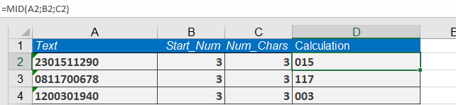

Additional Examples:

• =MID(« intercontinentalflight »; 1; 5)→ inter
• =MID(« gazelle »; 1; 4)→ gaze
• =MID(« gazelle »; 4; 4)→ elle
• =MID(« Louis »; 2; 3)→ oui
• =MID(« Excel »; 1; 2)→ Ex
• =MID(« Excel »; 2; 3)→ xce

This function converts a string to lowercase.

Syntax
LOWER(text)

Arguments

• text(required): The text you want to convert to lowercase.

Background
The LOWER() function is the counterpart of the UPPER() function, which converts a string to uppercase. All uppercase letters are converted to lowercase, while other characters (numbers, symbols, etc.) remain unchanged.

This function is useful for:

• Comparing strings in a non–case-sensitive manner.
• Standardizing text data to lowercase format.

If a numeric value is passed as the text argument, Excel converts it to unformatted text. However, if the result is used in numeric calculations, Excel automatically converts it back to a number.

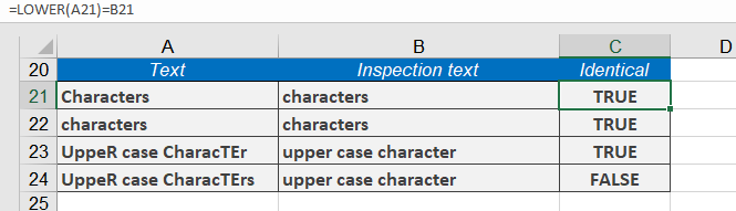
Example
To perform a case-insensitive comparison, you can convert text to lowercase. For example:

• =LOWER(« Letters »)= »letters »returns TRUE.
• =LOWER(« LETTERS »)= »letters »also returns TRUE.

Additional Examples

• =LOWER(« John Smith »)returns john smith.
• =LOWER(« Excel »)returns excel.
• =LOWER(« eXCEL »)returns excel.
• =LOWER(TODAY())returns 40450.