Votre panier est actuellement vide !
Catégorie : Excel function
How to use the HLOOKUP function in Excel
This function searches for a value in the top row of a table or array and returns a corresponding value from the specified row.
Syntax:
HLOOKUP(lookup_value; table_array; row_index_num; [range_lookup])
Arguments:
- lookup_value (optional): The value to search for (text, number, or logical value).
- table_array (required): A cell range or array constant (enclosed in braces {}).
- row_index_num (required): A positive integer indicating which row to return (must not exceed the table’s rows).
- range_lookup (optional):
- FALSE → Searches for an exact match.
- TRUE or omitted → Finds the nearest match (≤ lookup_value).
Background:
- Exact Match (range_lookup = FALSE):
- Searches the top row for an exact match of lookup_value.
- Returns #N/A if no match is found.
- No sorting required.
- Approximate Match (range_lookup = TRUE or omitted):
- Returns an exact match if found; otherwise, the largest value ≤ lookup_value.
- Requires the top row to be sorted in ascending order.
Example:
A bus timetable requires finding minutes based on a stop (column) and time (row) as seen in the table below.
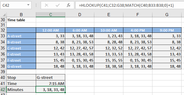
Since HLOOKUP() alone cannot handle row selection dynamically, combine it with MATCH():
=HLOOKUP(C41; C32:G38; MATCH(C40; B33:B38; 0) + 1)
- MATCH(C40; B33:B38; 0): Finds the stop (C40) in the first column.
- +1: Adjusts for the header row in table_array.
How to use the COLUMNS function in Excel
This function returns the number of columns in an array or cell reference.
Syntax:
COLUMNS(array)
Arguments:
- array (required): An array constant or a reference to a cell range.
Background:
- Using a discontiguous range as an argument triggers the error:
« You’ve entered too many arguments to the function. »
- Enclosing such arguments in extra parentheses results in a #REF! error.
- If the range is defined by intersections and the intersection is empty, the function returns #NULL!.
Array constants are numbers or text that you must enclose in braces. Rows are separated by semicolons, and columns are separated by commas
- {1;2;3;4} → Interpreted as a single column:
=COLUMNS({1;2;3;4}) // Returns 1
- {11,12,13;21,22,23} → Interpreted as three columns:
=COLUMNS({11,12,13;21,22,23}) // Returns 3
Example:
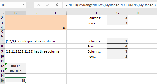
Combined with ROWS(), this function helps access specific cells in a named range, particularly useful for dynamic ranges.
- If a range is named MyRange, the formula:
=INDEX(MyRange; ROWS(MyRange); COLUMNS(MyRange))
Returns a reference to the lower-right cell of the range.
How to use the COLUMN function in Excel
This function returns the column number of a given cell reference.
Syntax:
COLUMN([reference])
Arguments:
- reference (optional): Must evaluate to a cell reference or range.
Background:
- If the reference argument is omitted, the function returns the column number of the cell containing the formula.
- If reference is a range (or a named range), the function can be used in array formulas:
- If the output range has fewer columns than the input, excess data is truncated.
- If the output range has more columns than the input, extra cells display #N/A.
Example:
Suppose you want to sum numbers in a row based on whether their column numbers are even or odd.
- A number is even if:
(2 * INT(A1 / 2) – A1) = 0 → TRUE
- A number is odd if:
(2 * INT(A1 / 2) – A1) <> 0 → TRUE
If cells B21:E21 contain numbers:
- Sum of even columns:
{=SUM((INT(COLUMN(B21:E21)/2)*2 – COLUMN(B21:E21) = 0) * B21:E21)}
- Sum of odd columns:
{=SUM((INT(COLUMN(B21:E21)/2)*2 – COLUMN(B21:E21) <> 0) * B21:E21)}
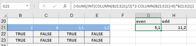
This works because Excel interprets:
- TRUE as 1
- FALSE as 0
How to use the CHOOSE function in Excel
This function uses an index to return a value from the list of value arguments.
Syntax:
CHOOSE(index; value1; value2; …)Arguments:
- index (required): Specifies which item is selected from the value arguments.
- value1, value2, … (the first value argument is required): A list of values separated by commas. These can be numbers, cell references, defined names, formulas, functions, or text.
- In Excel the maximum number of arguments is 254.
- In earlier versions, the limit is 29.
Background:
- The index argument must evaluate to an integer between 1 and 29 (or 1 and 254, depending on the Excel version).
- You can use a formula or a cell reference that returns such a number.
- If index is less than 1 or greater than the number of value arguments, CHOOSE() returns the #VALUE! error.
- If index is a fraction, the decimal part is truncated before evaluation.
Using CHOOSE() in Array Formulas:
You can use CHOOSE() in an array formula by specifying the index as an array. However, be cautious to avoid errors.- The formula:
{=CHOOSE({1;2}; SUM(E41:G41); SUM(E42:G42))}
Returns:
-
- The sum of E41:G41 in the first cell.
- The sum of E42:G42 in the second cell.
- The formula:
{=SUM(CHOOSE({1;2}; E41:G41; E42:G42))}
Returns the total of E41:G42 in both cells.
- The formulas:
=SUM(CHOOSE(1; E41:G41; E42:G42))
and
=SUM(CHOOSE(2; E41:G41; E42:G42))
Return the correct individual sums.
Example:
Assume the names of the days (starting with Sunday) are in cells B42:B48. The formula:= »Today is » & CHOOSE(WEEKDAY(D42); B42; B43; B44; B45; B46; B47; B48) & « . »
Returns:
« Today is [weekday name]. »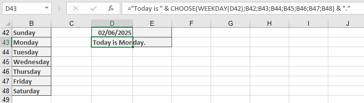
How to use the AREAS function in Excel
This function returns the number of contiguous ranges within a reference.
Syntax:
AREAS (reference)Arguments:
- reference (required): Must evaluate to a reference for one or more cell ranges. Otherwise, Excel returns an error (preventing formula entry) or an error value.
Background:
If the argument consists of multiple references separated by a comma, additional parentheses must be used:=AREAS((A1;A2))
or
=AREAS((A1:A2;B3))
If additional parentheses are omitted, the comma is treated as a list separator, resulting in an error. Attempting to calculate empty ranges returns the #NULL! error (e.g., =AREAS(A1 A2)), as no intersection exists between A1 and A2.
Example:
This function is not commonly used in daily Excel tasks but can be helpful when:- A dynamic list is named using the OFFSET() function.
- A list is formatted as a table.
Scenario:
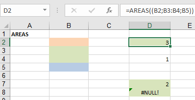
Suppose you want to expand a list by adding cells below its title while ensuring it does not exceed 100 entries. If row 100 is reached, the title row should change color as an alert.To count overlapping ranges between the named range List and cell A101, use:
=AREAS(List others!$A$101)
If the result is 1 (indicating an overlap), conditional formatting should change the title row’s colour. However, the Conditional Formatting dialog does not support intersection operations (spaces in cell references).
Workaround:
- Assign a name to the formula:
- In Excel: Formulas > Defined Names > Define Name.
- In Excel: Insert > Name > Define.
- Enter a reference name (e.g., Formula).
- Apply the conditional format to the title row using:
=(Formula=1)
and specify the desired colour.
How to use the ADDRESS function in Excel
Creates a cell reference as text from given row and column numbers.
Syntax:
ADDRESS(row_num; column_num; [abs_num]; [a1];[sheet_text])Arguments:
- row_num (required):
- Row number (1 to 1,048,576 in modern Excel)
- column_num (required):
- Column number (1 to 16,384 in modern Excel)
- abs_num (optional): Reference type:
- 1 [Default]: Absolute ($A$1)
- 2: Absolute row, relative column (A$1)
- 3: Relative row, absolute column ($A1)
- 4: Relative (A1)
- a1 (optional):
- TRUE/1: A1-style (default)
- FALSE/0: R1C1-style
- sheet_text (optional):
- Worksheet name (e.g., « Sheet2 ») to prefix reference
Key Notes:
- Truncates decimal values in row/column numbers
- Doesn’t verify worksheet existence
- Returns text, not an actual reference (use with INDIRECT() for dynamic references)
Examples
- Basic References
Formula Result =ADDRESS(6, 2) $B$6 =ADDRESS(6, 2, 4) B6 =ADDRESS(6, 2, 2) B$6 =ADDRESS(6, 2, , , « Sheet2 ») Sheet2!$B$6 - Automatic Column Labels
=LEFT(ADDRESS(1, COLUMN()-COLUMN($C$14)+1, 4), 1)
- Generates letters (A, B, …) for columns starting at C14
- COLUMN() calculates current column position
- Dynamic Cell Access
=INDIRECT(ADDRESS(6, 2)) // Returns value from B6
- Last Cell in Range
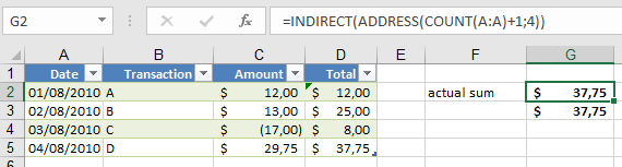
=INDIRECT(ADDRESS(COUNT(A:A)+1, 4))
- Finds last numeric entry in column A and returns value from column D
- For cross-sheet reference:
=INDIRECT(ADDRESS(COUNT(Payments!A:A)+1, 4,,, »Payments »))
Practical Applications
- Dynamic Headers:
Create self-updating column labels when columns are added/removed. - Summary Sheets:
Reference data from variable-length lists without manual updates. - Template Building:
Generate formulas that adapt to changing data structures. - Cross-Sheet References:
Programmatically create references to other worksheets.
Combination Techniques
- With MATCH()/INDEX():
=INDIRECT(ADDRESS(MATCH(« Total »,A:A,0), 2))
- With VLOOKUP():
=VLOOKUP(« Item », A:B, 2, 0) // Alternative to ADDRESS+INDIRECT
Limitations
- Reference strings may break if rows/columns are deleted
- Volatile when combined with INDIRECT()
- Consider INDEX() as a more stable alternative for many use cases
- row_num (required):
How to use the VALUE function in Excel
The VALUE() function converts text representations of numbers into numeric values.
Syntax:
VALUE(text)Arguments:
- text (required): The text string (enclosed in quotation marks) or cell reference containing the text to be converted to a number.
Background:
While Excel automatically converts number-like text to numeric values in most cases, the VALUE() function is particularly useful when:- Processing data imported from external sources (e.g., text files, databases)
- Handling numbers stored as text by third-party applications or add-ins
- Preparing data for mathematical operations where text-formatted numbers would cause errors
Alternative Conversion Method (Paste Special):
- Enter 1 in an empty cell and copy it (Ctrl+C)
- Select the range containing text-formatted numbers
- Use Paste Special (Home → Paste dropdown → Paste Special)
- Select Values and Multiply, then click OK
- Delete the temporary cell containing 1
Note: The VALUE() function supports all Excel-recognized formats for:
- Numbers (including decimals and currency symbols)
- Dates
- Times
Returns #VALUE! error for incompatible formats (e.g., logical values, text strings).
Examples
Formula Result Explanation =VALUE(« 1.234 ») 1234 Converts numeric text to number (uses system decimal separator) =VALUE(1234) 1234 Returns number unchanged =VALUE(« 09/09/2008 ») 39700 (date serial value) Converts date string to Excel date number =VALUE(TRUE) #VALUE! Fails with logical values =VALUE(« $1,000 ») 1000 Handles currency symbols and commas =VALUE(« 12:30 PM ») 0.520833 (time serial value) Converts time text to decimal 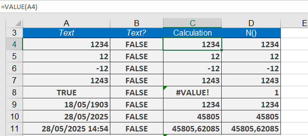
Key Notes
- Regional Settings Impact:
- Decimal/thousand separators must match system settings (e.g., VALUE(« 1,234 ») fails if system uses commas as decimals).
- Error Handling:
- Wrap with IFERROR for problematic data:
=IFERROR(VALUE(A1), « Invalid number »)
- Wrap with IFERROR for problematic data:
- Automatic Conversion:
- Excel usually auto-converts text to numbers in calculations (making VALUE() redundant in simple cases).
- Date/Time Caveat:
- Converted dates/times appear as serial numbers—apply number formatting to display properly.
Practical Use Case
When importing CSV data with numeric columns flagged as text:
=VALUE(TRIM(A2))
→ Combines TRIM() to remove extra spaces before conversionHow to use the UPPER function in Excel
This function converts all lowercase letters in a text string to uppercase.
Syntax:
UPPER(text)Arguments:
- text (required): The text you want to convert to uppercase.
Background:
The UPPER() function is useful for:- Standardizing text data (e.g., converting names or codes to uppercase)
- Case-insensitive comparisons in formulas
- Preparing text for case-sensitive systems
Key Notes:
- Only affects alphabetic characters (a-z → A-Z)
- Leaves numbers, symbols, and existing uppercase letters unchanged
- Returns text values (even if input appears numeric)
Examples
Formula Result Explanation =UPPER(« Letters ») « LETTERS » Converts all letters to uppercase =UPPER(« letters ») « LETTERS » Same as above =UPPER(« Excel ») « EXCEL » Standardizes mixed case =UPPER(« eXCEL ») « EXCEL » Converts all letters regardless of original case =UPPER(« 1,232.56 ») « 1,232.56 » Numbers and punctuation remain unchanged 
Limitations
- Does not affect non-alphabetic characters
- Returns text values (may require VALUE() wrapper for numeric operations)
- For proper capitalization (e.g., « John Smith »), use PROPER() instead
How to use the TRIM function in Excel
This function removes all spaces from text except for single spaces between words.
Syntax:
TRIM(text)Arguments:
- text (required): The text containing leading, trailing, or excessive intermediate spaces you want to clean.
Background:
The TRIM() function is particularly useful for:- Processing text imported from other applications that may contain irregular spacing
- Preparing data for mail merges or text searches where extra spaces could cause errors
- Cleaning datasets while preserving intentional single spaces between words
Unlike the Find and Replace command (Ctrl+H), TRIM() specifically targets:
→ Leading spaces (at the start of text)
→ Trailing spaces (at the end of text)
→ Multiple consecutive spaces between words (reducing them to single spaces)If the input string has no excess spaces, TRIM() returns the original text unchanged.
Examples
Formula Result Explanation =TRIM(« August ») « August » No spaces to remove =TRIM(« August « ) « August » Removes 1 trailing space =TRIM( » August ») « August » Removes 2 leading spaces =TRIM( » August « ) « August » Removes 1 leading + 2 trailing spaces =TRIM( » August the Strong « ) « August the Strong » Reduces multiple spaces between words to singles + removes leading/trailing spaces 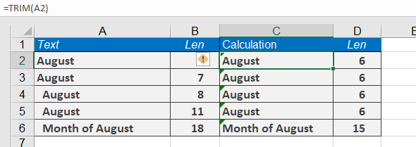
Practical Use Case
After importing data from a CSV file, you notice entries like:
» Product A » (with irregular spacing)Solution:
=TRIM(A1) converts this to « Product A » – clean and ready for analysis.Note: Unlike some string functions, TRIM():
✓ Preserves meaningful single spaces between words
✗ Doesn’t affect non-breaking spaces (ASCII 160) – use SUBSTITUTE() for thoseKey Takeaways
- Essential for data cleaning, especially with imported text
- Only affects space characters (ASCII 32)
- Returns text values (wrap with VALUE() if numbers need conversion)
How to use the TEXT function in Excel
This function converts a value into text in a specific number format.
Syntax:
TEXT(value; format_text)Arguments:
- value (required): A number, a formula that evaluates to a numeric value, or a reference to a cell containing a numeric value.
- format_text (required): A number format, which is one of those in the Custom category box on the Number tab in the Format Cells dialog box.
Background:
You might need to convert numeric values to text to link static text with calculations. The TEXT() function not only converts numeric values to text but also allows you to use the number formats available in the Format Cells dialog box.In the format_text argument, you can specify custom formats. However, the formats have the following restrictions:
- Formats cannot contain an asterisk (*).
- The General number format is not allowed.
- Colors (e.g., red for negative values) are ignored.
The difference between the Format Cells command and the TEXT() function is that TEXT() returns text. A number formatted with Format Cells remains a numeric value. You can still use numbers converted with TEXT() in other formulas because Excel automatically converts text-formatted numbers back to numeric values for calculations.
Examples
- Dynamic Payment Date in an Invoice
To display a payment due date (14 days from today) in a readable format:
Formula:
=CONCATENATE(« Please pay before « ; TEXT(TODAY()+14; « MM/DD/YYYY »); ». »)Result :
« Please pay before 06/DD/YY. »Without TEXT():
=CONCATENATE(« Please pay before « ; TODAY()+14; « . »)
Result: « Please pay before 40527. » (Excel’s date serial number, which is unreadable to users).- Current Date in a Sentence
To format today’s date as a full sentence:
Formula:
= »Today is » & TEXT(TODAY(); « DDDD ») & « , » & TEXT(TODAY(); « MMMM D; YYYY ») & « . »Result (May 28, 2025):
« Today is Wednesday, may 28, 2025. »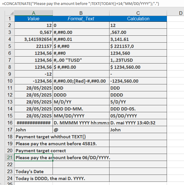
Key Notes
- Use TEXT() to force a specific format (e.g., dates, currency) when combining numbers with text.
- Avoid using TEXT() for calculations, as it converts numbers to strings (though Excel may auto-convert them back in formulas).
- For standalone number formatting (without text concatenation), Format Cells is preferable.