Votre panier est actuellement vide !
Étiquette : practical-excel
Inserting Sparklines in Excel
Are you looking for a way to visualize a large volume of data in a small space? Sparklines are a quick and elegant solution. These mini-charts are specifically designed to show data trends inside a single cell.
Creating a Sparkline Chart
A sparkline chart is a small chart that resides in a single cell. The idea is to place a visual next to the original data without taking up too much space, which is why sparklines are sometimes called “inline charts.” Sparklines can be used with any numerical data in a tabular format. Typical uses include visualizing temperature fluctuations, stock prices, periodic sales figures, and any other time-based variation.
You insert sparklines next to rows or columns of data and get a clear graphical presentation of a trend in each individual row or column.
Sparklines were introduced in Excel 2010 and are available in all later versions: Excel 2013, Excel 2016, Excel 2019, and Excel for Microsoft 365.
To create a sparkline in Excel, follow these steps:
- Select a blank cell where you want to insert a sparkline, typically at the end of a data row.
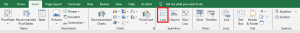
- On the Insert tab, in the Sparklines group, choose the desired type: Line, Column, or Win/Loss.
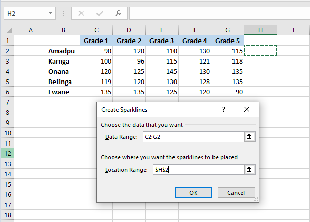
- In the Create Sparklines dialog box, place your cursor in the Data Range box and select the range of cells to include in the sparkline.
- Click OK.
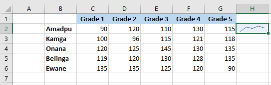
And there you have it – your very first mini-chart appears in the selected cell. Want to see how the data evolves in other rows? Simply drag the fill handle to instantly create a similar sparkline for each row in your table.
Adding Sparklines to Multiple Cells
In the previous example, you learned one way to insert sparklines into multiple cells: add it to the first cell and copy it. Alternatively, you can create sparklines for all the cells at once. The steps are exactly the same as described above, except you select the full range instead of a single cell. Here are the detailed instructions:
- Select all the cells where you want to insert mini-charts.
- Go to the Insert tab and choose the desired sparkline type.
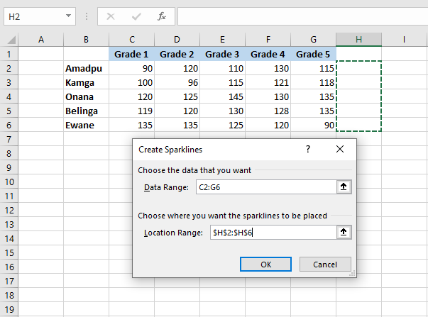
- In the Create Sparklines dialog box, select all the source cells for the Data Range.
- Make sure Excel displays the correct location range where your sparklines should appear.
- Click OK.
Types of Sparklines
Microsoft Excel provides three types of sparklines: Line, Column, and Win/Loss.
Line Sparklines
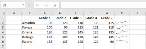
These sparklines look very similar to tiny line charts. Like traditional line charts in Excel, they can be drawn with or without markers. You are free to modify the line style as well as the line and marker colors. We’ll cover how to do that later. For now, here’s an example of line sparklines with markers: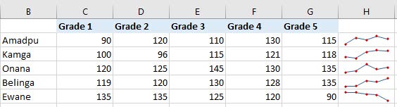
Column Sparklines
These tiny charts appear as vertical bars. Just like a standard column chart, positive data points are above the x-axis and negative ones are below. Zero values are not shown – a blank space is left for a zero data point. You can set the color of your choice for positive and negative mini-columns, and highlight the highest and lowest points.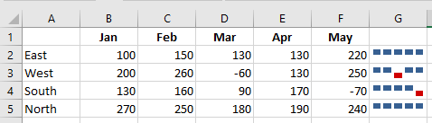
Win/Loss Sparklines
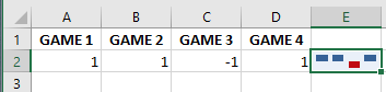
This type resembles a column sparkline but does not show the magnitude of a data point – all bars are the same size regardless of the original value. Positive values (wins) are plotted above the x-axis and negative values (losses) below. A Win/Loss sparkline can be thought of as a binary micro-chart, best used with values that have only two states such as True/False or 1/-1. For example, it works perfectly to display game results where 1s represent wins and -1s losses: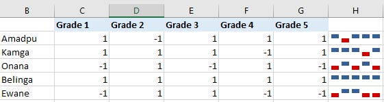
Editing Sparklines
After creating a sparkline in Excel, what’s the next thing you’d usually want to do? Customize it to your liking! All customization is done via the Design tab that appears once you select an existing sparkline in a sheet.
Changing the Sparkline Type
To quickly change the type of an existing sparkline:
- Select one or more sparklines in your worksheet.
- Go to the Design tab.
- In the Type group, choose the desired type.
Showing Markers and Highlighting Specific Data Points
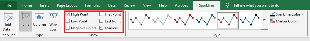
To make the most important points in your sparklines more visible, you can highlight them in a different color. You can also add markers for each data point. Just select the desired options on the Sparkline tab, in the Show group:
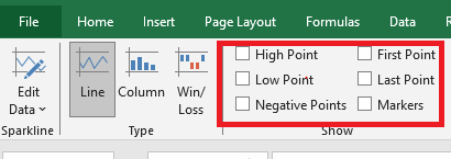
Available options include:
- High Point – highlights the maximum value.
- Low Point – highlights the minimum value.
- Negative Points – highlights all negative values.
- First Point – highlights the first data point.
- Last Point – changes the color of the last data point.
- Markers – adds markers to each data point (available only for line sparklines).
Changing Sparkline Color, Style, and Line Width
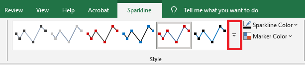
To change the appearance of your sparklines, use the style and color options on the Design tab in the Style group:
- To apply a built-in sparkline style, select it from the gallery. To see all styles, click the More button in the lower-right corner.
- To change the default color, click the arrow next to Sparkline Color and pick your preferred color.
- To adjust line thickness, click the Weight option and choose from preset widths or set a custom thickness (available only for line sparklines).
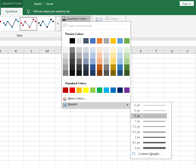
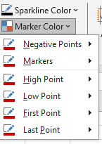
- To change marker color or specific data point colors, click the arrow next to Marker Color and select the desired item:
Customizing the Sparkline Axis
By default, Excel sparklines are drawn without axes or coordinates. However, you can display a horizontal axis if needed and perform a few other customizations. Details are provided below.
How to Change the Axis Starting Point
By default, Excel draws a sparkline so that the smallest data point appears at the bottom, and all other points are scaled relative to it.
In some situations, this can be misleading — it may give the impression that the lowest data point is near zero and that the variation among data points is greater than it actually is. To fix this, you can make the vertical axis start at 0 or at any value you consider appropriate.
To do so, follow these steps:
- Select your sparklines.
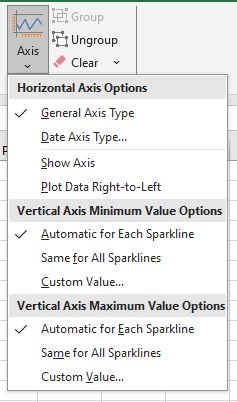
- On the Design tab, click the Axis button.
- Under Vertical Axis Minimum Value Options, select Custom Value…
- In the dialog box that appears, enter 0 or another minimum axis value you prefer.
- Click OK.
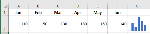
The image below shows the result — by forcing the sparkline to start at 0, we now get a more realistic picture of the variation between data points:
Note: Be very careful with axis customizations when your data contains negative numbers — if you set the vertical axis minimum to 0, all negative values will disappear from the sparkline chart.
How to Show the X-Axis in a Sparkline
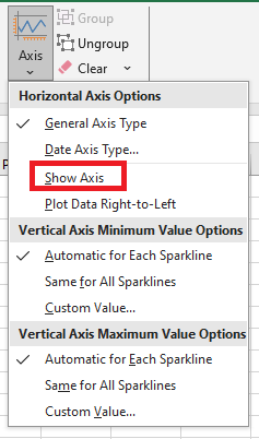
To display a horizontal axis in your micro-chart, select it, then click Axis > Show Axis on the Sparkline tab.
This works best when data points fall on both sides of the x-axis — that is, when you have both positive and negative numbers:
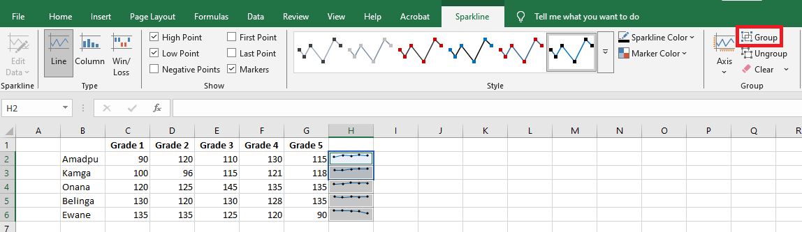
How to Group and Ungroup Sparklines
When you insert multiple sparklines in Excel, grouping them gives you a major advantage: you can change the entire group at once.
To group sparklines, do the following:
- Select two or more mini-charts.
- On the Design tab, click the Group button.
To ungroup sparklines, select them and click the Ungroup button.
Note: When you insert sparklines into multiple cells, Excel automatically groups them.
How to Resize Sparklines
Because Excel sparklines are background images inside cells, they resize automatically to fit the cell.
- To change the width of sparklines, make the column wider or narrower.
- To change the height, increase or decrease the row height.
How to Delete a Sparkline
When you decide to remove a sparkline that you no longer need, you may be surprised to find that pressing the Delete key does nothing.
Here are the steps to delete a sparkline in Excel:
- Select the sparkline(s) you want to remove.
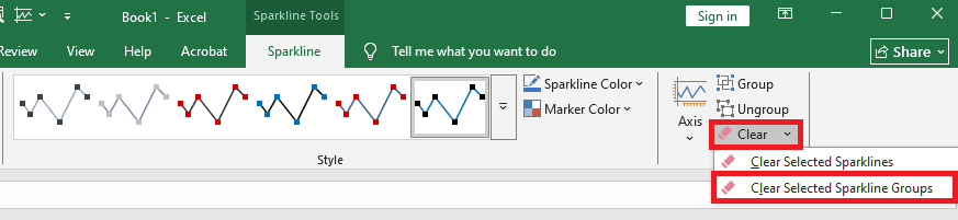
- On the Design tab, do one of the following:
- To delete only the selected sparkline(s), click the Clear button.
- To delete the entire group, click Clear > Clear Selected Sparkline Groups.
Tip: If you accidentally deleted the wrong sparkline, press Ctrl + Z to undo the action.
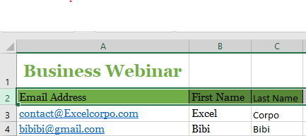
Applying Cell Styles in Excel
To apply multiple formatting attributes in a single step and ensure consistency across your cells, you can use a cell style. A cell style is a predefined set of formatting characteristics, such as font and font size, number formats, cell borders, and shading.
To prevent changes to specific cells, you can also use a cell style that locks the cells.
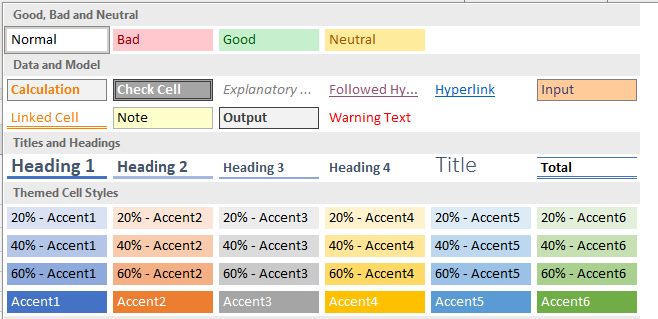
Microsoft Excel includes several built-in cell styles that you can apply or modify. You can also edit or duplicate a cell style to create your own custom style.
NOTE
Cell styles are based on the document theme applied to the entire workbook. When you change the document theme, the cell styles are automatically updated to match the new theme.
We use cell styles to apply consistent formatting such as fonts, font sizes, cell borders, cell shading, and number formats. In this tutorial, we’ll learn how to apply, create, and delete a cell style.
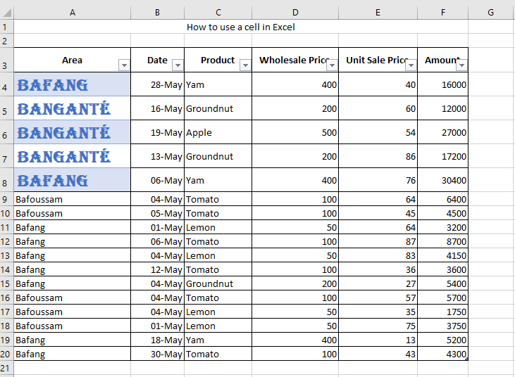
How to Apply a Cell Style
We can apply a Title or Total cell style using the following steps:
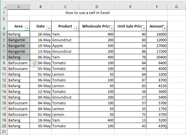
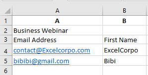
■ Select the cells, rows, or columns you want to format.
In this case, we select A4:A8 from our data.
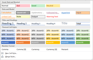
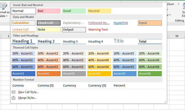
■ Go to the Home tab and click More in the Styles group.
■ In the drop-down list, choose the style you want and click Apply.
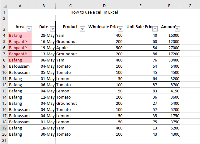
■ We will apply the Bad cell style, and the result will look like this:
How to Create a Custom Cell Style
■ Select the cells where you want to apply the custom style.
In this case, we select A3:A8.
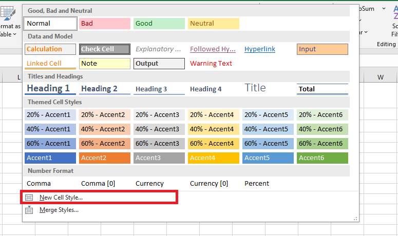
■ Go to the Home tab and click the More drop-down arrow in the Styles group.
■ At the bottom, click New Cell Style.
■ In the Style name box, enter an appropriate name for the new style.
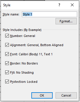
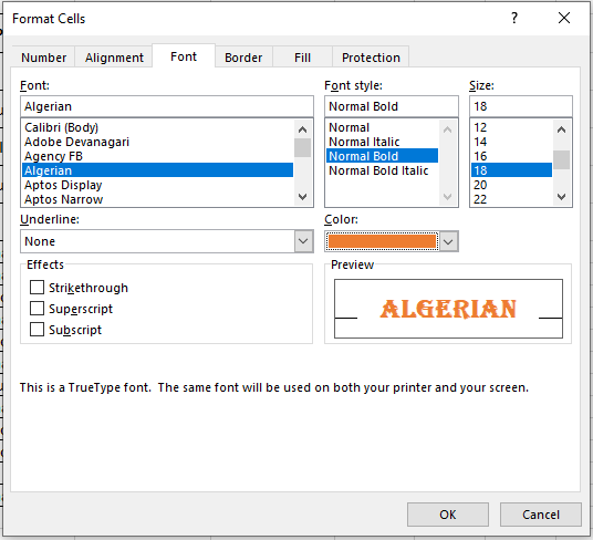
■ Then, under the style name, click Format.
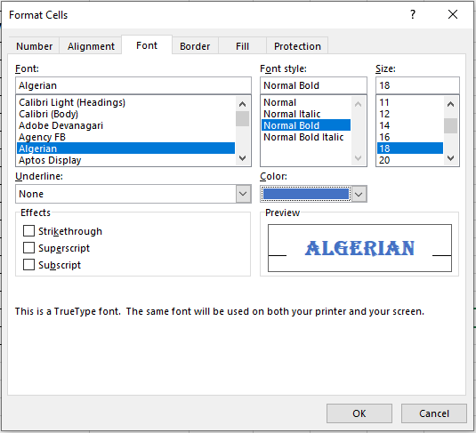
In the Format Cells dialog box, choose the font and colors you want, then click OK.
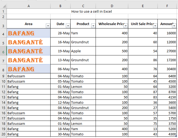
■ In the Style dialog box, under Style includes (example), uncheck any formatting you don’t want included.
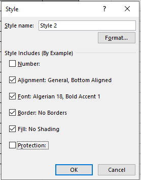
■ Click OK.
You can now apply your new custom cell style, just like any other built-in style.
How to Create a Cell Style by Modifying an Existing One
■ In the Home tab, click the More drop-down arrow in the Styles group.
■ Then do one of the following:- Right-click on an existing cell style and choose Modify.
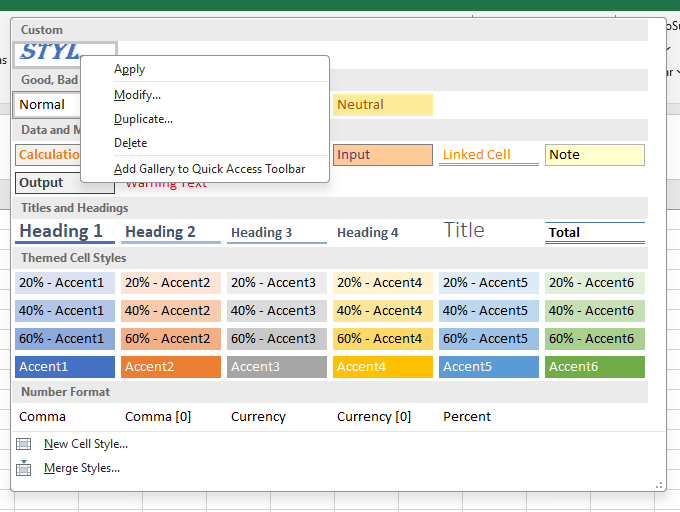
- Or right-click on a style and select Duplicate to create a copy.
■ In the Modify Cell Style dialog box, click Format.
In the various tabs of the Format Cells dialog box, choose the desired formatting and click OK.
■ In the Style dialog box under Style includes, check or uncheck the boxes for any formatting you want to include or exclude.
Applying Cell Formats in Excel
All cell contents initially use the same default formatting, which can make it difficult to read a workbook with a lot of information. Basic formatting helps personalize the appearance of your workbook, allowing you to draw attention to specific sections and make your content easier to read and understand.
You can also apply number formatting to tell Excel exactly what type of data you’re using in your workbook, such as percentages (%), currency ($), and more.
Changing the Font
By default, the font in every new workbook is set to Calibri. However, Excel offers many other fonts to help you customize the text in your cells.
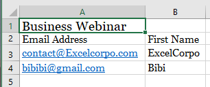
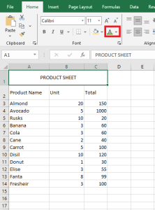
In the example below, we’ll format the title cell to distinguish it from the rest of the worksheet.
- Select the cell(s) you want to modify.
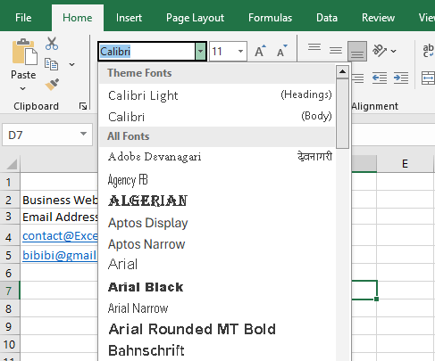
- Click the drop-down arrow next to the Font command on the Home tab.
The font menu will appear. - Select the desired font. A live preview will appear as you hover over different options.
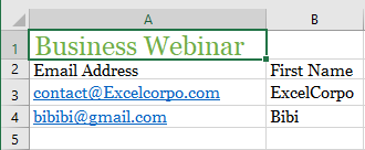
In our example, we’ll choose Georgia.
- The text will update to the selected font.
For professional workbooks, choose an easy-to-read font. Besides Calibri, good options include Cambria, Times New Roman, and Arial.
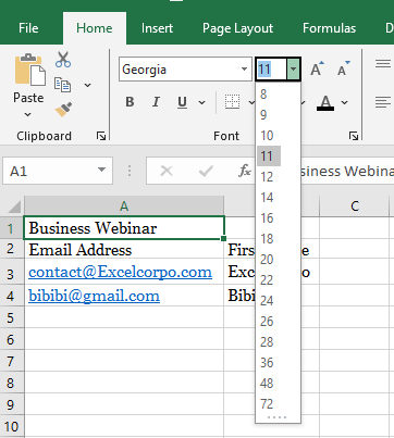
Changing the Font Size
- Select the cell(s) you want to modify.
- Click the drop-down arrow next to the Font Size command on the Home tab.
The font size menu will appear. - Select the desired font size. A live preview will appear as you hover.
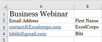
In our example, we’ll choose 16 to enlarge the text.
- The text will update to the selected size.
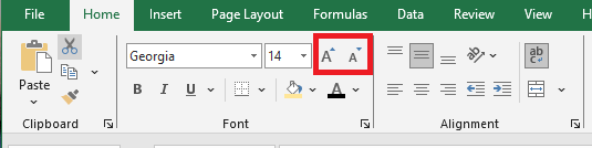
You can also use the Increase Font Size and Decrease Font Size buttons or type a custom size using your keyboard.
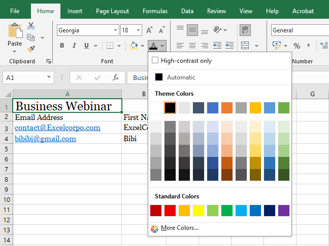
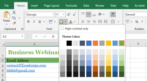
Changing the Font Color
In Excel, you can add visual interest by changing the font color. While spreadsheets are often used to display specific data, that doesn’t mean they have to look plain. Adding a touch of color can make your sheets more appealing and easier to read.
You can choose a theme color, a standard Excel palette color, or create a custom one.
- Select the cell(s) you want to modify.
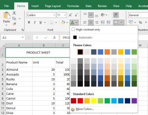
- Click the drop-down arrow next to the Font Color command on the Home tab.
The color menu will appear. - Select the desired color. A live preview appears as you hover.
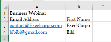
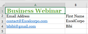
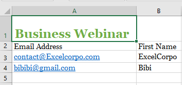
In our example, we’ll choose Green.
- The text will update to the selected color.
To access more color options, click More Colors at the bottom of the menu.
Adding a Background Color to a Cell Range
You can make a range stand out by applying a background color.
If you want to change the background color based on cell values (e.g., red for negative, green for positive), conditional formatting is more suitable.
You can use a theme color, a standard color, or a custom one.
- Select the range you want to format.
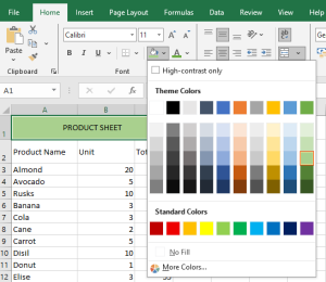
- Click the Home tab.
- Click the Fill Color drop-down list.
- Click a theme color or a standard color.
Excel applies the fill color to the selected range.
To remove the background color, select No Fill.
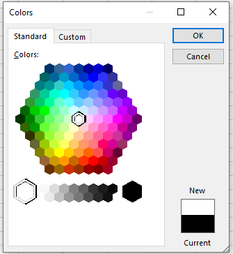
To use a custom color:
- Select the range.
- Go to Home > Fill Color > More Colors.
- Choose a color or click the Custom tab to adjust RGB values.
- Click OK.
Using Bold, Italic, and Underline Commands
To enhance appearance and impact, apply text effects like:
- Bold: to highlight labels
- Italic: to emphasize text
- Underline: for titles and headers
- Select the cell(s) you want to modify.

- Click the Bold (B), Italic (I), or Underline (U) button on the Home tab.
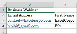
In our example, we’ll bold the selected cells.
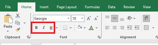
- The selected effect will apply to the text.
You can also use keyboard shortcuts:
- Ctrl+B = Bold
- Ctrl+I = Italic
- Ctrl+U = Underline
Text Alignment
By default:
- Text is bottom-left aligned
- Numbers are bottom-right aligned
You can change alignment to improve readability.
Horizontal alignment:
- Left Align: aligns content to the cell’s left edge
- Center Align: centers content horizontally
- Right Align: aligns content to the right
Vertical alignment:- Top Align: aligns content to the top
- Middle Align: centers content vertically
- Bottom Align: aligns content to the bottom
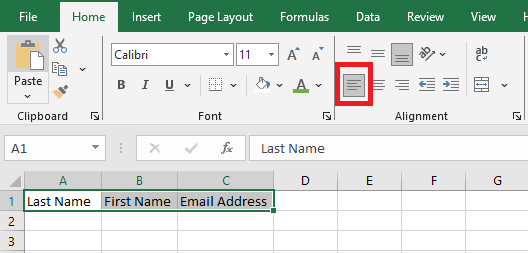
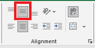
To apply horizontal alignment:
- Select the cell(s).
- On the Home tab, click one of the three horizontal alignment buttons.
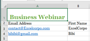
In our example, we select Center Align.
- The text realigns accordingly.
To apply vertical alignment:
- Select the cell(s).
- Choose one of the three vertical alignment options.
In our example, we choose Middle Align.
- The text is realigned.
You can combine both vertical and horizontal alignment.
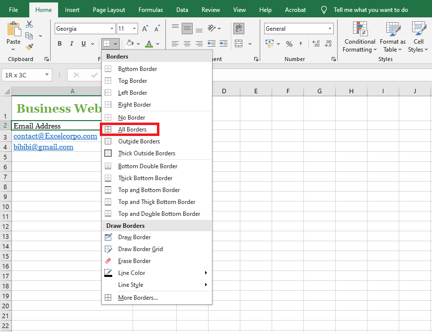
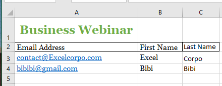
Cell Borders and Fill Colors
Cell borders and fill colors help define clear boundaries in your spreadsheet. Below, we’ll apply both to header cells.
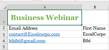
To add a border:
- Select the cell(s).

- Click the Borders drop-down arrow on the Home tab.
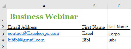
The border menu appears. - Select a border style (e.g., All Borders).
- The selected border appears.
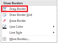
To customize line style and color, use the Draw Borders tools at the bottom of the menu.
To add a fill color:
- Select the cell(s).
- Click the Fill Color drop-down on the Home tab.
- Choose a color. Live preview is available.
In our example, we select Light Green.
The fill color is applied.
Applying Number Formats in Excel
When you enter a number in a cell, you can display that number in a variety of different formats. Excel has quite a few built-in number formats, but sometimes none of them are exactly what you need. This chapter explains how to create custom number formats and provides many examples that you can use as-is or adapt to your needs.
About Number Format
By default, all cells use the General number format (what you type is what you get). But if the cell is not wide enough to display the entire number, the General format rounds decimal numbers and uses scientific notation for large numbers. In many cases, the General number format works just fine, but most people prefer to specify a different number format for better consistency.
Excel automatically applies a built-in number format to a cell based on the following criteria:
■ If a number contains a slash (/), it may be converted to a date or fraction format.
■ If a number contains a dash (-), it may be converted to a date format.
■ If a number contains a colon (:) or is followed by a space and the letter A or P (uppercase or lowercase), it may be converted to a time format.
■ If a number contains the letter E (uppercase or lowercase), it may be converted to scientific notation (also called exponential format). If the number doesn’t fit the column width, it may also be converted to this format.Formatting Numbers Using the Ribbon
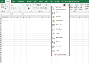
The Number group on the Home tab of the Ribbon contains several commands for quickly applying common number formats. The Number Format drop-down menu gives you quick access to 11 common number formats.
Additionally, the Number group contains a few buttons. When you click one of these buttons, the selected cells adopt the specified number format. The table below summarizes the formats these buttons apply.
Shortcut Applied Formatting Ctrl+Shift+~ General format (unformatted values) Ctrl+Shift+$ Currency format with two decimal places (negative numbers appear in parentheses) Ctrl+Shift+% Percentage format with no decimals Ctrl+Shift+^ Scientific notation format with two decimal places Ctrl+Shift+# Date format with day, month, and year Ctrl+Shift+@ Time format with hour, minute, and AM/PM Ctrl+Shift+! Two decimals, thousand separator, dash for negative values Using the Format Cells Dialog Box to Format Numbers
For maximum control over number formatting, use the Number tab in the Format Cells dialog box. You can access this dialog box in several ways:
■ Click the dialog box launcher in the lower-right corner of the Number group on the Home tab.
■ Choose Home / Number / Number Format / More Number Formats.
■ Press Ctrl+1.
The Number tab of the Format Cells dialog box contains 12 number format categories to choose from. When you select a category in the list box, the right side of the dialog updates to display the appropriate options.
Here are the number format categories, along with some general comments:
■ General: Default format; displays numbers as integers, decimals, or scientific notation if the value is too wide for the cell.
■ Number: Specify decimal places, whether to use the system’s thousands separator (e.g., a comma), and how to display negative numbers.
■ Currency: Specify decimal places, choose a currency symbol, and display negative numbers. This format always uses the system’s thousands separator.
■ Accounting: Similar to Currency but aligns currency symbols vertically, regardless of the number of digits.
■ Date: Choose from a variety of date formats and select regional settings for date formatting.
■ Time: Choose from a variety of time formats and select regional settings for time formatting.
■ Percentage: Choose the number of decimals; always displays a percent sign.
■ Fraction: Choose from nine fraction formats.
■ Scientific: Displays numbers in exponential notation (with an E): e.g., 2.00E+05 = 200,000. You can choose the number of decimal places to show before the E.
■ Text: When applied, Excel treats the value as text (even if it looks like a number). Useful for things like numeric part numbers or credit card numbers.
■ Special: Contains additional formats. The list varies based on the selected locale. For U.S. English, formatting options include ZIP Code, ZIP+4, phone number, and Social Security number.
■ Custom: Define number formats not included in the other categories.NOTE
If a cell displays a series of hash marks (such as #########) after you apply a number format, this usually means the column is not wide enough to display the value using the selected format. Widen the column (by dragging the right border of the column header) or change the number format. A series of hash marks can also mean the cell contains an invalid date or time.
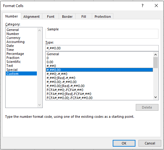
Creating a Custom Number Format
When you create a custom number format, it can be used to format any cell in the workbook.
You can create about 200 custom number formats per workbook. The following figure shows the Custom category in the Number tab of the Format Cells dialog box.
You can create number formats not included in the other categories. Excel gives you great flexibility in defining custom number formats.
Custom number formats are stored in the workbook in which they are defined. To make a custom format available in another workbook, simply copy a cell using the custom format to the other workbook.
Parts of a Numeric Format String
Number format codes are strings of symbols that define how Excel displays the data stored in cells. We’ll explain how to write formats, but first we need to clarify how Excel interprets these symbols.
Each numeric format code can contain up to four sections, separated by semicolons (;), allowing you to specify different format codes for positive numbers, negative numbers, zero values, and text. The codes follow this order:
Positive Format ; Negative Format ; Zero Format ; Text Format
If you don’t use all four sections in a format string, Excel interprets it as follows:
■ If you use only one section: it applies to all numeric values.
■ If you use two sections: the first applies to positive values and zeros, the second to negative values.
■ If you use three sections: the first applies to positives, the second to negatives, and the third to zeros.
■ If you use all four sections: the last applies to text stored in the cell.You can choose to skip formatting for any section by entering
General. For example, if you only want to format positive numbers and text, you could use a format string like:Section1; General; General; Section4
Note that
Generalremoves any special formatting from the data entered—so be careful. Negative numbers usingGeneralwill not display a minus sign.Custom Number Format Codes
The table below lists formatting codes for custom formats, along with brief descriptions.
Code Description General Displays the number in General format. # Placeholder for optional digits. If not needed, the digit is not shown. Used for more readable numbers. 0 Placeholder for mandatory digits. Even if a digit is not significant, it will display. Example: 0.00always shows two decimals., (comma) Indicates the location of the decimal or thousands separator. % Percentage format. (space) Thousand separator placeholder. Helps define behavior for thousands/millions. E-, E+, e-, e+ Scientific notation. \ Displays the character following the backslash as-is. ? Placeholder that aligns decimals by spacing insignificant zeros. Useful in fractions. * Repetition modifier. Used with a character to fill the cell with that character. _ (underscore) Space modifier. Inserts a space equal to the width of the specified character. Useful for aligning parentheses. « text » Displays the text within double quotes. @ Text placeholder. [Color] Displays characters in a specified color. [Color n] Displays the corresponding color from the palette (n = 0 to 56). [Condition] Sets your own condition for each section of a number format.
Example 1: Changing Font Color
One of the simplest things you can do with number format codes is change the font color. The syntax is:
[ColorName]For example, you can assign a different color for each section of the format string:
[Red]General;[Blue]General;[Magenta]General;[Cyan]General
This results in:

Note that the negative number in line 3 no longer displays a minus sign. Also, color formatting does not affect decimal places or text alignment.
Example 2: Adding Text with Format Codes
You can add text to numbers using format codes in two ways:
Single characters: To prefix a symbol like
@, type a backslash (\) followed by the symbol.Example:
\@General
Results in output: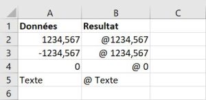
Full text strings: To append text like « units », enclose the string in double quotes:
Example:
General" units"
Results in output:
If extended to all four sections like this:
General" units"; General" units"; General" units"; General" units"Then the output looks like:
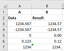
Example 3: Zero (0)
Here is an example using the zero placeholder. The following format:
0.00Ensures that numbers always display with two decimal places, even if the decimal part is zero.
Merci pour la suite du texte. Je vais maintenant te fournir la traduction complète en anglais de cette nouvelle section, en conservant le style technique du guide Excel.
Zeros in a number format code represent mandatory digits.
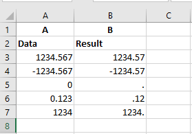
Example 4: Question Mark (?)
Here is an example of the question mark code in action. The following format code is used:
0,??
A question mark is a placeholder for a digit. It adds space for insignificant zeros on either side of the decimal point so that decimals align properly when using a fixed-width font.
Example 5: Hash Symbol (#)
Here is an example of the hash symbol code in action. The following format code is used:
#, ##
The hash symbol represents an optional digit. If the digit is not needed, it will not be displayed in the formatted number.
Example 6: Space
Here is an example of the space code in action. The following format is used:
$??? ???,00
The space character in number format codes acts as a placeholder for thousands separators.
Example 7: Asterisk (*)
Here is an example of the asterisk code in action. The following format is used:
*=0.##
The asterisk is a repeating character modifier. It repeats the character to fill the remaining width of the cell.
Example 8: Underscore (_)
Here is an example using the underscore code. Format used:
_(#,##_);(#,##)
The underscore creates a blank space equal to the width of the character following it. It is useful for aligning positive and negative numbers, especially when negative values use parentheses.
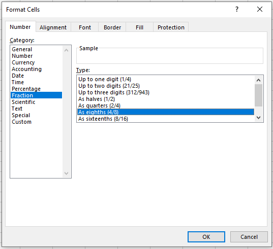
Example 9: Fractions ( / )
Excel supports several built-in fraction formats (found under the « Fraction » category in the Format Cells dialog box). For example, to display 0.125 as an eighth, select As eighths (4/8) from the Type list.
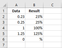
Fractions are special because they involve unit conversion. For example:
- 0.23 is shown as 23/100,
- 0.25 can be simplified to 1/4,
- 1.25 can be shown as 1 1/4 or 5/4.
Excel rounds to the closest fraction based on the format code and follows the same rules as the hash and question mark symbols.
Mixed Fractions (Integer with Reduced Fraction)
A typical format separates the integer part from the fractional part. Use question marks for better alignment:
#???/???
This preserves the alignment of the fraction bar regardless of digit count. For example:
#??/??
Displays 0.23 as 3/13 instead of 23/100.Improper Fractions
If you prefer to merge the whole number into the fraction:
###/###This creates an improper fraction format with up to three digits.
Fixed-Base Fractions
To force Excel to round to a fixed denominator, include it in the format code:
###/15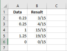
The value is rounded to the nearest 15th.
Example 10: Percentages (%)
Like fractions, percentages are controlled by format codes. A simple format might be:
#%
You can also specify fractional percentages:
##/#%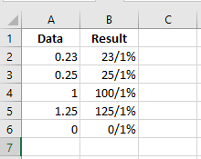
This shows percentages as simplified fractions.
You can also include decimals:
#,0%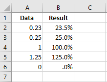
Example 11: Scientific Notation (E)
Large or tiny numbers are difficult to read with standard notation. Scientific notation shifts the decimal point for clarity:
- 0.0000001 becomes 1 × 10⁻⁷
- Excel shows this as
1E-07
The capital letter E signals scientific notation.
A format like
#E+#shows the base and exponent, while:0.00E+00
forces both parts to show two digits.

This provides consistent display with predictable string length.
Scaling Values
Custom formats can also scale numbers. For instance, you might want to display numbers in thousands or millions, while preserving the actual value for calculations.
Displaying Thousands
Format:
# ###(space at the end)This removes the last three digits and rounds to the nearest integer.
Format:
# ###,00
Rounds to two decimals.Value Format Display 123456 # ###123 1234565 # ###1,235 -323434 # ###–323 123123.123 # ###123 499 # ###1 123456 # ###,00123.46 499 # ###,000.50
Displaying Hundreds
Format:
0","00
Divides by 100 and displays two decimals.Value Format Display 546 0","005.46 500 0","005.00 -500 0","00–5.00
Displaying Millions
Format:
# ###(two spaces)
or# ###,00
or# ### "M"
or complex format:
# ###,0 "M"_);(# ###,0 "M)";0,0"M"_Value Format Display 123456789 # ###123 1.23457E+11 # ###123,457 5000000 # ###,005.00 -5000000 # ###,00–5.00 0 # ###,000.00 1000000 # ### "M"1M 0 # ###,0 "M"_);(# ###,0 "M)";0,0"M"_0.0M –5000000 same complex format (5.0M)
Custom Date and Time Format Codes
Code Description m Month (1–12, no leading zero) mm Month (01–12) mmm Abbreviated month (Jan, Feb) mmmm Full month name d Day (1–31, no leading zero) dd Day (01–31) ddd Abbreviated weekday (Mon, Tue) dddd Full weekday (Monday, Tuesday) yy Year (2 digits) yyyy Year (4 digits) h Hour (0–23, no leading zero) hh Hour (00–23) s Second (0–59) ss Second (00–59) [ ] Display times above 24h or minutes >60 AM/PM 12-hour clock \ Escapes next character . Decimal point « text » Displays quoted text Dates entered are formatted based on the system’s short date. This can be adjusted in Windows settings.
Value Format Display 42552 mmmm d, yyyy (dddd)July 1, 2016 (Friday) 42552 "Today is" dddd!Today is Friday! 42552 dddd, mm/dd/yyyyFriday, 07/01/2016 0.345 h:mm "hours"8:16 hours 0.78 h:mm a/p".m."6:43 p.m. Conditional Format Specification
The following format displays different text depending on the cell’s value:
[<10]"Too Low";[>10]"Too High";"Just Right"- If value < 10 → displays “Too Low”
- If value > 10 → displays “Too High”
- If value = 10 → displays “Just Right”
Note: Only one or two conditions are allowed, plus a default fallback.
In most cases, Excel’s built-in Conditional Formatting feature is a better solution for value-based styling.
Wrapping Text Automatically in Cells in Excel
If you have text that is too wide to fit within the column but you don’t want it to spill over into adjacent cells, you can use the Wrap Text option to fit the text within the cell.
The Wrap Text option displays the content across multiple lines within the same cell, if necessary. Use this option to display long headings without having to widen columns or reduce text size.
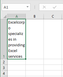
- For example, look at the long string of text in cell A1 below. Cell B1 is empty.
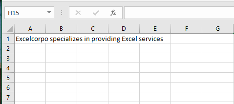
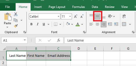
- On the Home tab, in the Alignment group, click Wrap Text.
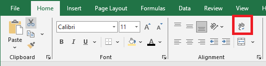
Result:
- Click the right border of column header A and drag the separator to increase the column width.
- Double-click the bottom border of row header 1 to automatically adjust the row height.
To insert a manual line break, follow these steps:
- For example, double-click in cell A1.
- Place your cursor at the position where you want the line to break.
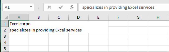
- Press Alt + Enter.
Formatting Cells Using the Format Painter Tool in Excel
When it comes to copying formatting in Excel, Format Painter is one of the most useful — yet often underused — features. This tool copies the formatting from one cell and applies it to other cells. In just a few clicks, it can help you reproduce most, if not all, formatting settings, including:
- Number formats (General, Percentage, Currency, etc.)
- Font, size, and color
- Font attributes such as bold, italic, and underline
- Fill color (background color of the cell)
- Text alignment, direction, and orientation
- Cell borders
To use the Format Painter tool, follow these steps:
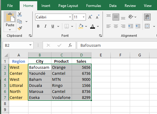
- Select the text or graphic that has the formatting you want to copy.
- On the Home tab, click Format Painter.
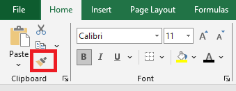
The pointer changes to a paintbrush icon.- Use the brush to « paint » over a selection of text or graphics to apply the formatting. This works only once.
If you want to apply the formatting to multiple selections, first double-click the Format Painter button.
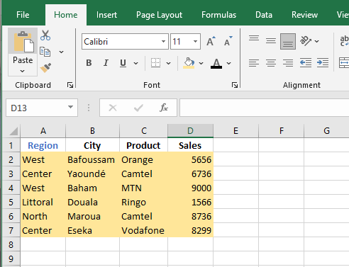
- To stop formatting, press ESC.
Changing Cell Alignment and Orientation in Excel
The content of a cell can be aligned both horizontally and vertically. By default, Excel aligns numbers to the right and text to the left. All cells use bottom alignment by default.
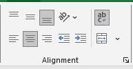
The most commonly used alignment commands are located in the Alignment group on the Home tab of the ribbon.
To change text alignment:
- Select the relevant cells and activate the Home tab. Then go to the Alignment group.
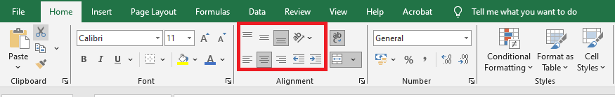
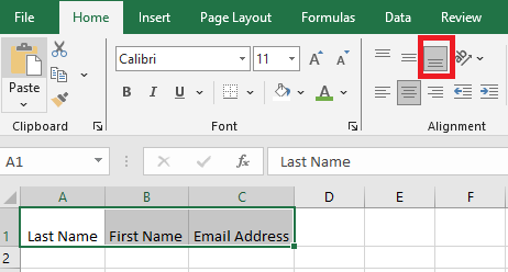
- To change the vertical alignment of the cell content relative to the row height, click one of the following tools in the Alignment group:
- Top Align
- Middle Align
- Bottom Align
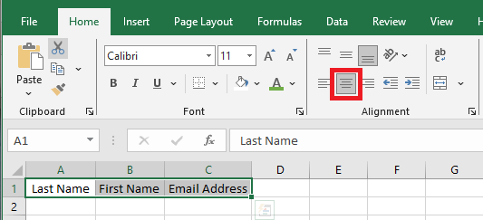
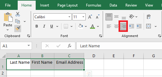
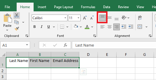
- To change the horizontal alignment of the cell content relative to the column width, click one of the following tools:
- Align Left
- Center
- Align Right
If you want to change how the data appears in a cell, you can rotate the font angle or modify the text alignment. To do this:
- Select a cell, row, column, or range.
- Go to Home > Orientation, then choose an option.
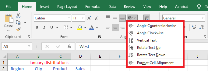
You can rotate your text up, down, left, or right, or align it vertically:
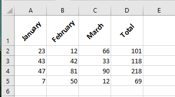
To rotate text to a specific angle:
- Select a cell, row, column, or range.
- Go to Home > Orientation > Format Cell Alignment.
- Under Orientation on the right-hand side, in the Degrees box, use the up or down arrow to set the exact number of degrees to rotate the cell’s text.
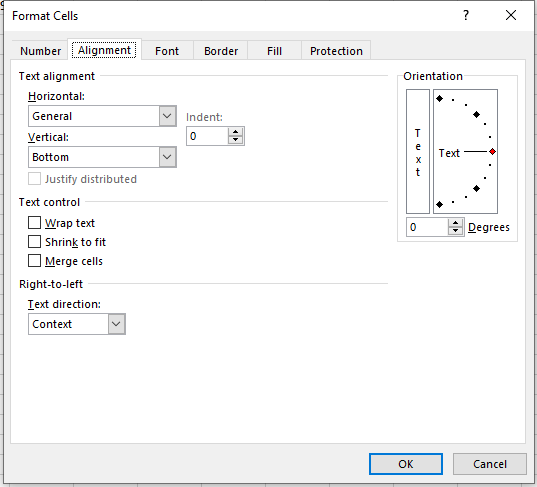
- Positive numbers rotate the text upward.
- Negative numbers rotate the text downward.
Horizontal Alignment Options
Horizontal alignment options control how the content is distributed across the width of the cell (or cells). They are available in the Format Cells dialog box:
- General: Aligns numbers to the right, text to the left, and centers logical and error values. This is the default setting.
- Left (Indent): Aligns content to the left side of the cell. If the text is wider than the cell, it overflows into the cell on the right. If the right cell isn’t empty, the text is cut off. Also available on the ribbon.
- Center: Centers the content within the cell. If the text is too wide, it overflows into adjacent empty cells; otherwise, it is truncated. Also available on the ribbon.
- Right (Indent): Aligns content to the right side. If the text is too wide, it overflows to the left if the adjacent cell is empty. Also available on the ribbon.
- Fill: Repeats the content to fill the width of the cell. If adjacent cells to the right are also set to Fill, they will also be filled.
- Justify: Justifies the text left and right across the cell. Applies only if the cell is set to wrap text and spans multiple lines.
- Center Across Selection: Centers the text across selected columns. Useful for centering a title across multiple columns.
- Distributed: Distributes the text evenly across the selected column.
Vertical Alignment Options
Vertical alignment options are not used as often as horizontal ones. They are mostly useful when row height has been increased significantly.
Here are the vertical alignment options available in the Format Cells dialog box:
NOTE:
If you choose Left, Right, or Distributed, you can also adjust the Indent setting, which adds horizontal spacing between the cell border and the text.
- Top: Aligns cell content at the top of the cell. Also available on the ribbon.
- Center: Vertically centers the content in the cell. Also available on the ribbon.
- Bottom: Aligns content to the bottom of the cell. Also available on the ribbon.
- Justify: Justifies the text vertically within the cell; this applies only when the cell uses wrap text and multiple lines. This setting can increase line spacing.
- Distributed: Distributes the text evenly vertically in the cell.
Merging Cells in Excel
Excel allows you to merge cells, columns, and rows to combine numbers, text, or other data to effectively organize your information. Merging cells helps structure your data, making it easier to read and understand.
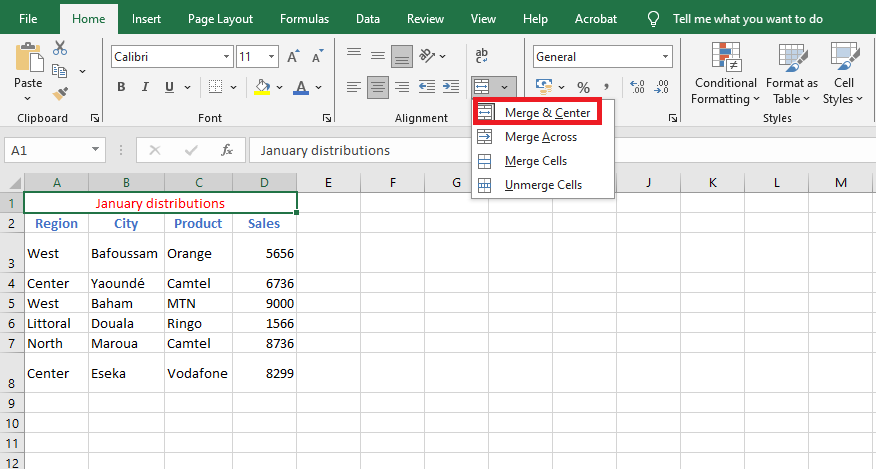
To merge a cell in Excel, use the drop-down list located in the Alignment group on the Home tab, as shown in the figure below.
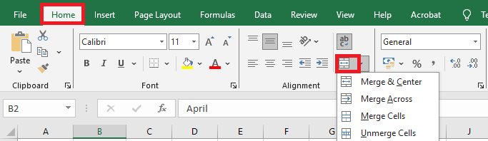
The merge drop-down list contains various merge options that allow you to combine multiple cells into a single one.
The different options in the Merge & Center drop-down list are explained as follows:
- Merge & Center: This merges the selected cells and centers the data string in the new merged cell. During the merge, only the content of the leftmost cell is preserved; the contents of the other merged cells are deleted.
- Merge Across: This merges the selected cells in each row individually (across columns). It keeps only the content of the leftmost cell in each row.
- Merge Cells: This merges all the selected cells into a single cell. The selected range can be horizontal, vertical, or both. Only the content of the upper-left cell is retained.
- Unmerge Cells: This reverses the merge operation, splitting the merged cells back into individual cells.
NOTE:
The difference between Merge & Center and Merge Cells lies in the alignment: the former centers the content, the latter does not.
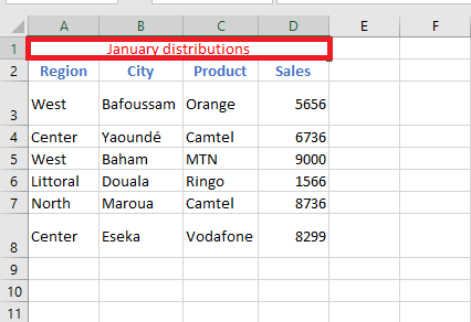
One of the main reasons to merge multiple cells is to create a title row in your worksheet.
To merge and center multiple cells:
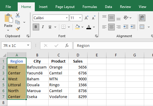
- Select all the cells you want to merge and center so they span the width of your data table.
- Then, go to the Home tab, click on the Merge & Center drop-down, and select the first option: Merge & Center.

As shown, all your cells are merged, and the heading “January Distributions” is centered at the top of the table. You can also merge cells vertically.
If you try to merge multiple rows, multiple columns, or both rows and columns, only the content from the top-left cell of the selection will be kept; all others will be discarded.
To merge several rows and columns:
- Select the cells, open the Merge & Center drop-down menu, then click on the Merge & Center option.
All the selected cells will then be merged into a single cell, and the value from the top-left cell will be centered in the resulting merged cell.

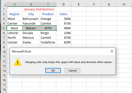
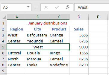
If you select multiple columns and choose Merge Cells from the Merge & Center menu, all values except those in the leftmost cells will be lost. Excel will display a warning before proceeding.
As you can see, all the columns are now combined into a single cell, without centering the text.
The second option in the drop-down list, Merge Across, works similarly to the third option, Merge Cells, but it merges the selected cells in each row separately. This only works on horizontal (row-wise) cell selections.
Inserting and Deleting Cells in Excel
Inserting Cells
When working in an Excel worksheet, you may need to insert or delete cells without inserting or deleting entire rows or columns.
To insert cells:
- Select the location where the new cells will be inserted. This can be a single cell or a range of cells.
- Right-click and choose Insert.
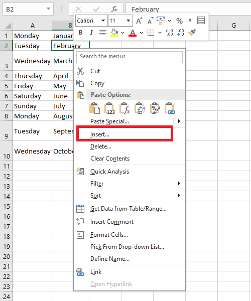
- The Insert dialog box opens. Select either:
- Shift cells right to move the cells in the same row to the right.
- Shift cells down to move the selected cells and all cells below in the column downward.
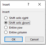
- Choose an option, then click OK.
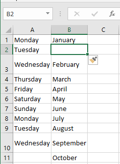
- Your result appears in the worksheet.
Note: You can also use the Insert dialog box to insert or delete entire rows and columns.
Deleting Cells
To delete a cell from the worksheet:
- Right-click and choose Delete.
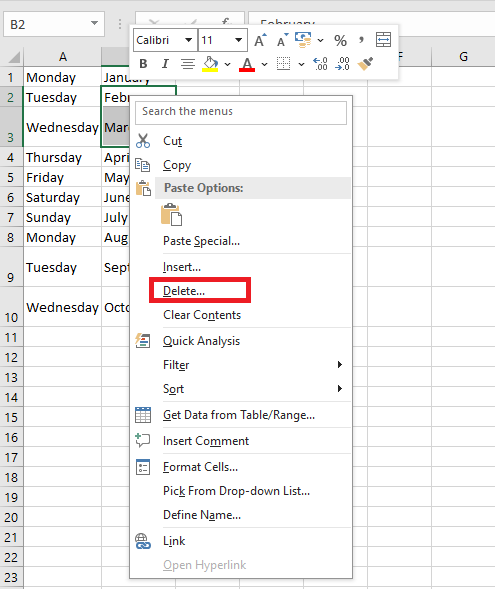
- The Delete dialog box opens. Select either:
- Shift cells left to move the cells in the same row to the left.
- Shift cells up to move the selected cells and all cells below upward.
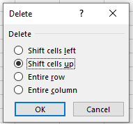
- Choose an option, then click OK.
- Your result is displayed in your worksheet.
NOTE
You can also Insert or Delete a cell from the Cells group items on the Home tab.Deleting the Contents of a Cell Range
Deleting a range actually removes the cells from the worksheet.
NOTE
You can also insert or delete a cell using the Cells group on the Home tab.
However, if you want the cells to remain but want to remove their contents or formatting, you can use Excel’s Clear command, as described in the following steps:
- Select the range you want to clear.
- Select Home > Clear. Excel displays a submenu with clear options.
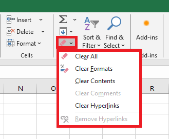
- Select Clear All, Clear Formats, Clear Contents, Clear Comments, or Clear Hyperlinks, as appropriate.
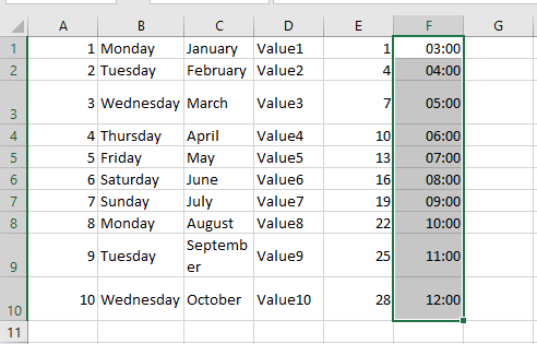
To clear values and formulas from a range using the fill handle, you can use either of the following two methods:
- If you want to clear only the values and formulas from a range, select the range, then click and drag the fill handle across the range and over the cells you want to clear. Excel shades the cells as you select them. When you release the mouse button, Excel clears the values and formulas from the cells.
- If you want to clear everything in the range — such as values, formulas, formats, and comments — select the range, then hold down the Ctrl key. Next, click and drag the fill handle across the range and over each cell you want to clear. Excel clears the cells when you release the mouse button.
Filling Cells Using AutoFill in Excel
The fill handle is the small black square in the lower-right corner of the active cell or range. This small, versatile tool can do many useful things, including creating a series of text or numeric values and filling, clearing, inserting, and deleting ranges. The following sections show you how to use the fill handle to perform each of these tasks.
Using AutoFill to Create Text and Number Series
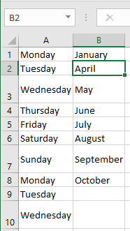
Worksheets often use text series (such as January, February, March, or Sunday, Monday, Tuesday) and numeric series (such as 1, 3, 5 or 2009, 2010, 2011). Instead of entering these series manually, you can use the fill handle to create them automatically. This handy feature is called AutoFill. The following steps show how it works:
- For a text series, select the first cell of the range you want to use and enter the initial value. For a numeric series, enter the first two values, then select both cells.
- Position your mouse pointer over the fill handle. The pointer changes to a plus sign (+).
- Click and drag the mouse pointer until the gray border surrounds the range you want to fill. If you’re unsure where to stop, watch the tooltip near the mouse pointer showing the value of the last selected cell.
- Release the mouse button. Excel fills the range with the series.
When you release the mouse button after using AutoFill, Excel not only fills the series but also displays the Auto Fill Options smart tag. To view the options, move your cursor over the smart tag and click the down arrow to open the list. The options you see depend on the type of series you created. However, you will typically see at least the following four:
- Copy Cells: Click this option to fill the range by copying the original cell(s).
- Fill Series: Click this option for the default series fill.
- Fill Formatting Only: Click this to apply only the formatting from the original cell to the selected range.
- Fill Without Formatting: Click this to fill the range with series data but without copying the formatting.
Keep the following guidelines in mind when using the fill handle to create series:
- Dragging the fill handle down or to the right increments values. Dragging it up or to the left decrements values.
- The fill handle recognizes standard abbreviations like Jan (January) and Sun (Sunday).
- To change the series interval for a text series, enter the first two values, then select both before dragging. For example, entering 1st and 3rd produces the series 1st, 3rd, 5th, and so on.
Creating a Custom AutoFill List
As you saw in the previous sections, Excel recognizes some values such as January, Sunday, or Qtr1 as part of larger predefined lists. When you drag AutoFill from a cell containing one of these values, Excel fills the cells with the appropriate series. However, you are not limited to Excel’s built-in lists. You are free to define your own AutoFill lists as described in the following steps:
- Select File > Options to open the Excel Options dialog box.
- Click Advanced, then click Edit Custom Lists to open the Custom Lists dialog box.
- In the Custom lists box, click New List. A cursor appears in the List entries box.
- Type an item for your list in the List entries box and press Enter. Repeat this step for each item. (Make sure to enter the items in the order you want them to appear in the series.)
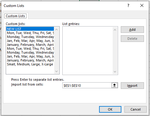
If you need to delete a custom list, select it in the Custom Lists box and click Delete.
If you already have the list in a worksheet range, don’t bother entering each item manually. Instead, open the Import list from cells dialog and enter a reference to the range. You can type the reference or select the cells directly in the worksheet. Click the Import button to add the list to the Custom Lists box.
Using the Series Command
Instead of using the fill handle to create a series, you can use Excel’s Series command to gain a bit more control over the entire process. Follow these steps:
- Select the first cell you want to use for the series and enter the starting value. If you want to create a pattern-based series (like 2, 4, 6, etc.), fill in enough cells to define the pattern.
- Select the full range you want to fill.
- On the Home tab, choose Fill > Series in the Editing group. Excel displays the Series dialog box.
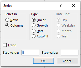
- Click Rows to create the series across rows from the active cell or click Columns to create the series down columns.
- Use the Type group to click your desired series type. You have the following options:
- Linear: This finds the next value in the series by adding the step value (see step 6) to the previous value.
- Growth: This finds the next value by multiplying the previous one by the step value.
- Date: This creates a date series based on the option you select in the Date unit group, such as Day, Weekday, Month, or Year.
- AutoFill: This works similarly to the fill handle. You can use it to extend a numeric pattern or a text series like Qtr1, Qtr2, Qtr3.
If you want to extend a trend, check the Trend box. You can only use this option with Linear or Growth series types.
- If you chose a Linear, Growth, or Date series type, enter a number in the Step value box. Excel uses this number to increment each value in the series.
- To set a limit on the series, enter the appropriate number in the Stop value box.
- Click OK. Excel fills the series and returns you to the worksheet.