Catégorie : Excel function

Its Calculates depreciation for an asset using the declining balance method, with an optional switch to straight-line depreciation when advantageous. This flexible approach is commonly used for tax purposes.

Syntax

VDB(Cost; Salvage; Life; Start_Period; End_Period; [Factor]; [No_Switch])

Arguments

Argument	Required	Description	Validation Rules
Cost	Yes	Initial asset value (purchase price + expenses).	Must be positive.
Salvage	Yes	Asset value at end of depreciation.	Must be ≥ 0 and < Cost.
Life	Yes	Useful life in periods (integer).	Must be > 0.
Start_Period	Yes	Starting period for depreciation calculation.	Must be < Life.
End_Period	Yes	Ending period for depreciation calculation.	Must be ≥ Start_Period.
[Factor]	No	Accelerated depreciation rate (default=2 for double-declining).	Typically 1.5–2.
[No_Switch]	No	FALSE (default): Switches to straight-line when optimal; TRUE: Forces declining balance.	Logical (TRUE/FALSE).

Error Conditions

• #VALUE!: Non-numeric inputs.
• #NUM!: If:
  • Cost ≤ 0 or Salvage < 0
  • Life ≤ 0 or Start_Period ≥ Life
  • Factor ≤ 0

Background

The Variable Declining Balance (VDB) method combines:

1. Accelerated Depreciation: Higher expenses in early years (e.g., double-declining balance).
2. Automatic Switch to Straight-Line: When straight-line depreciation exceeds the declining balance amount.

Key Formula

Depreciation=Book Value×(FactorLife)Depreciation=Book Value×(LifeFactor​)

• Book Value = Cost – Accumulated Depreciation.
• Switch Condition: If straight-line depreciation > declining balance, VDB switches.

Example

Asset Depreciation:

• Cost: $1,000
• Salvage: $100
• Life: 10 years
• Factor: 2 (double-declining)
• No_Switch: FALSE (auto-switch enabled)

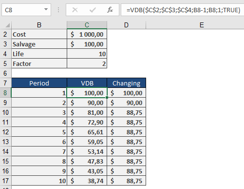
Depreciation Schedule

Year	Method	Depreciation	Book Value
1	Double-Declining	$200.00	$800.00
2	Double-Declining	$160.00	$640.00
3	Double-Declining	$128.00	$512.00
4	Straight-Line*	$103.00	$409.00
…	…	…	…

*Switches to straight-line in Year 4 when it becomes more beneficial.

Key Features

1. Tax Optimization: Maximizes early-year deductions.
2. Flexibility: Adjust Factor for local tax rules (e.g., 1.5× for mid-range acceleration).
3. Partial Periods: Combine with manual adjustments for mid-year purchases.

Complementary Functions

• DB(): Fixed declining balance (no switch).
• DDB(): Double-declining balance (no switch).
• SLN(): Straight-line depreciation.

Its calculates the yield to maturity of a U.S. Treasury bill (T-bill) as an annualized percentage, based on the purchase price and time to maturity.

Syntax

TBILLYIELD(Settlement; Maturity; Price)

Arguments

Argument	Required	Description	Validation Rules
Settlement	Yes	Trade settlement date (purchase date).	Must be valid date < Maturity.
Maturity	Yes	Maturity/redemption date.	Must be ≤ 1 year after Settlement.
Price	Yes	Purchase price per $100 face value.	Must be positive and < 100 (discounted).

Error Conditions

• #VALUE!: Invalid date format.
• #NUM!: If:
  • Settlement ≥ Maturity
  • Maturity > 1 year after Settlement
  • Price ≤ 0 or ≥ 100

Background

T-bills are zero-coupon securities sold at a discount. The yield represents the annualized return if held to maturity.

Key Formula

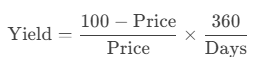
Where:

• Days = Actual calendar days between Settlement and Maturity.
• Uses 360-day year (consistent with U.S. banking conventions).

Example

T-Bill Investment:

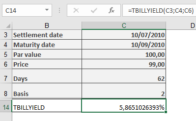
Key Notes

1. Comparison with Other Functions
   • YIELDDISC(Basis=2) matches TBILLYIELD().
   • RECEIVED() calculates maturity value, not yield.
2. Practical Use
   • Compare T-bill returns with other short-term investments.
   • Adjusts for the 360-day banking year (no compounding).
3. Limitations
   • Only valid for T-bills with maturities ≤ 1 year.
   • Price must be < 100 (discounted securities).

Its calculates the price per $100 face value of a U.S. Treasury bill (T-bill) based on its discount rate. T-bills are short-term securities that are issued at a discount and mature at par value.

Syntax

TBILLPRICE(Settlement; Maturity; Discount)

Arguments

Argument	Required	Description	Validation Rules
Settlement	Yes	The trade settlement date	Must be valid date < Maturity
Maturity	Yes	The maturity/redemption date	Must be ≤ 1 year after Settlement
Discount	Yes	The annual discount rate (decimal)	Must be > 0

Error Conditions

• #VALUE!: Invalid date format
• #NUM!: If:
  • Settlement ≥ Maturity
  • Maturity > 1 year after Settlement
  • Discount ≤ 0

Calculation Method

The price is calculated using:

Price = 100 × (1 – Discount × D/360)

Where:

• D = Number of days between Settlement and Maturity
• Uses actual calendar days (Basis = 2 equivalent)

Example

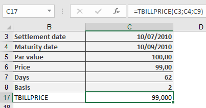
Key Features

1. Day Count Convention: Uses actual/360 (Basis = 2)
2. Output Format: Returns price as percentage of par value
3. Complementary Functions:
   • TBILLYIELD(): Calculates yield from price
   • PRICEDISC(): Similar but allows different day count bases

Its Calculates the bond-equivalent yield (annualized return) for a U.S. Treasury bill (T-bill) based on its discount rate, converting the T-bill’s discount yield (360-day basis) to an equivalent investment yield (365-day basis).

Syntax

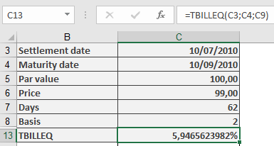
TBILLEQ(Settlement; Maturity; Discount)

Arguments

Argument	Required	Description	Validation Rules
Settlement	Yes	Trade date (when T-bill is purchased).	Must be a valid date < Maturity.
Maturity	Yes	Maturity date (when T-bill is redeemed).	Must be ≤ 1 year after Settlement.
Discount	Yes	Discount rate (as a decimal, e.g., 5% = 0.05).	Must be > 0.

Error Conditions

• #VALUE!: Invalid dates.
• #NUM!: If:
  • Settlement ≥ Maturity
  • Maturity > 1 year after Settlement
  • Discount ≤ 0

Background

T-bills are zero-coupon securities sold at a discount and redeemed at par. The TBILLEQ function converts the discount rate (used to price T-bills) into an equivalent annual yield (used to compare returns with other investments).

Key Formula

Where:

• Days = Actual days between Settlement and Maturity.

Example

Key Notes

1. Comparison with Other Functions
   • YIELDDISC(): Returns the yield directly (no 365-day conversion).
   • RECEIVED(): Calculates maturity value, not yield.
2. Practical Use
   • Compare T-bill returns with bonds or savings accounts.
   • Adjusts for the 360-day banking year used in T-bill pricing.
3. Limitations
   • Only valid for T-bills with maturities ≤ 1 year.
   • Does not account for compounding.

Its calculates the depreciation of an asset for a specified period using the sum-of-the-years’ digits (SYD) method, an accelerated depreciation technique that applies higher depreciation expenses in earlier periods.

Syntax

SYD(Cost; Salvage; Life; Per)

Arguments

Argument	Required	Description	Validation Rules
Cost	Yes	Initial asset cost (purchase price + additional expenses – discounts). Must be a positive value.	#VALUE! if non-numeric, invalid if negative.
Salvage	Yes	Asset value at the end of its useful life. Must be ≥ 0.	#VALUE! if non-numeric, #NUM! if negative.
Life	Yes	Total depreciation periods (integer > 0).	Must be a positive integer.
Per	Yes	Specific period for depreciation calculation (integer > 0).	Must be ≤ Life.

Background

Depreciation reflects the reduction in an asset’s value over time. The SYD method applies a declining depreciation expense each period, unlike straight-line depreciation.

Key Features

1. Accelerated Depreciation: Higher expenses in early years, decreasing over time.
2. Formula:

1. • Numerator: Remaining useful life at the start of the period.
   • Denominator: Sum of the years’ digits (e.g., 5 years → 1+2+3+4+5 = 15).
2. Tax & Accounting Use:
   • Permitted in some jurisdictions for tax benefits.
   • Not suitable for all assets (check local regulations).

Example

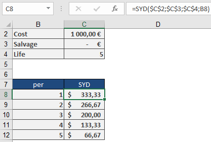
Asset Details:

• Cost: $1,000
• Salvage Value: $0
• Life: 5 years

Depreciation Schedule:

Year	Calculation (SYD)	Depreciation	Book Value
1	=SYD(1000,0,5,1)	$333.33	$666.67
2	=SYD(1000,0,5,2)	$266.67	$400.00
3	=SYD(1000,0,5,3)	$200.00	$200.00
4	=SYD(1000,0,5,4)	$133.33	$66.67
5	=SYD(1000,0,5,5)	$66.67	$0.00

Key Takeaway:

• Year 1 has the highest depreciation ($333.33).
• Year 5 has the lowest ($66.67).

Implementation Notes

1. Partial-Year Depreciation:
   • SYD assumes full periods. Adjust manually for mid-year purchases.
2. Complementary Functions:
   • SLN(): Straight-line depreciation.
   • DDB(): Double-declining balance (more aggressive than SYD).
3. Best Practices:
   • Use ROUND(SYD(…), 2) for financial reporting precision.
   • Verify tax compliance before applying SYD.

Its calculates straight-line depreciation for an asset over a specified period, allocating equal depreciation expense in each accounting period.

Syntax

SLN(Cost; Salvage; Life)

Arguments

Argument	Required	Description	Validation Rules
Cost	Yes	Initial asset value (purchase price + incidental costs)	Must be positive
Salvage	Yes	Asset value at end of depreciation	Must be ≥ 0
Life	Yes	Useful life in periods	Must be integer > 0

Error Conditions

• #VALUE!: Non-numeric inputs
• #NUM!: Negative values or invalid Life

Calculation Method

Annual Depreciation = (Cost – Salvage) / Life

Key Features

1. Equal Periodic Charges: Allocates depreciation evenly across all periods
2. Common Applications:
   • Financial reporting
   • Tax calculations (where permitted)
   • Budget forecasting

Example

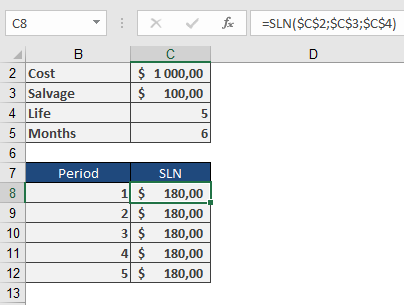
Asset Depreciation Scenario:

• Purchase cost: $1,000
• Salvage value: $100
• Useful life: 5 years

Calculation:

=SLN(1000, 100, 5)

Result: $180 per year

Depreciation Schedule:

Year	Beginning Value	Depreciation	Ending Value
1	$1,000	$180	$820
2	$820	$180	$640
3	$640	$180	$460
4	$460	$180	$280
5	$280	$180	$100

Implementation Notes

1. First-Year Convention:
   • For partial-year depreciation, manually adjust first period
   • Use SLN() for subsequent full periods
2. Best Practices:

=ROUND(SLN(Cost, Salvage, Life), 2)

Ensures compliance with financial reporting standards

1. Complementary Functions:
   • DB(): Declining balance method
   • DDB(): Double-declining balance
   • SYD(): Sum-of-years’ digits

Technical Considerations

1. Tax Compliance:
   • Verify local regulations permit straight-line method
   • Some jurisdictions require accelerated methods
2. Asset Management:
   • Combine with physical depreciation tracking
   • Useful for capital budgeting analysis

Its calculates the maturity value (redemption amount) for a fully discounted security that uses anticipative interest calculation (interest deducted upfront).

Syntax

RECEIVED(Settlement; Maturity; Investment; Discount; [Basis])

Arguments

Argument	Required	Description	Validation Rules
Settlement	Yes	Trade settlement date	Must be valid date ≤ Maturity
Maturity	Yes	Security maturity date	Must be valid date ≥ Settlement
Investment	Yes	Amount invested (purchase price)	> 0
Discount	Yes	Annual discount rate	> 0
[Basis]	No	Day count convention (0-4)	Default=0

Error Conditions

• #VALUE!: Invalid dates or non-numeric inputs
• #NUM!: Negative amounts or invalid Basis

Key Features

1. Anticipative Interest Model:
   • Interest deducted at inception (discount instrument)
   • Contrasts with standard arrears interest calculation
2. Common Applications:
   • Treasury bills
   • Commercial paper
   • Bankers’ acceptances

Calculation Method

Maturity Value = Investment / (1 – (Discount × DSM/DIM))

Where:

• DSM = Days from settlement to maturity
• DIM = Days in year per Basis convention

Examples

1. Bill of Exchange

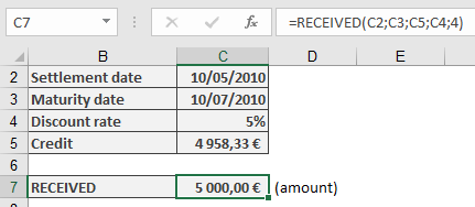
Scenario:

• Settlement: 10-May-2010
• Maturity: 10-Jul-2010 (2 months)
• Investment: $4,958.33
• Discount: 5% p.a.
• Basis: 4 (European 30/360)

Calculation:

=RECEIVED(« 5/10/2010″, »7/10/2010 »,4958.33,5%,4)

Result: $5,000.00

Face value of the bill

Important Notes

1. Day Count Conventions:

Basis	Method
0	US (NASD) 30/360
1	Actual/actual
2	Actual/360
3	Actual/365
4	European 30/360

1. Financial Context:
   • Primarily for short-term instruments (<1 year)
   • Represents the face value calculation
   • Complementary to PRICEDISC() which calculates purchase price
2. Implementation Tip:
   For precise institutional calculations:

=ROUND(RECEIVED(…), 2)

Related Functions

• PRICEDISC(): Calculates purchase price from face value
• YIELDDISC(): Determines equivalent yield
• INTRATE(): Calculates the interest rate

Its calculates the periodic interest rate for a loan or investment based on constant periodic payments and/or a lump sum amount.

Syntax

RATE(Nper; Pmt; Pv; [Fv]; [Type]; [Guess])

Arguments

Argument	Requirement	Description	Financial Context
Nper	Required	Total number of periods	Loan term/investment horizon
Pmt	Conditionally Required	Payment per period	Annuity amount
Pv	Conditionally Required	Present value	Loan principal/initial investment
[Fv]	Optional	Future value	Target balance/residual value
[Type]	Optional	Payment timing: 0 = end period (default) 1 = beginning period	Cash flow timing
[Guess]	Optional	Starting guess for iterative calculation (default=10%)	Initial estimate

Note: Either Pmt or Fv must be provided.

Calculation Method

Uses iterative approximation to solve the time value of money equation:

Pv + Σ[Pmt/(1+Rate)^k] + Fv/(1+Rate)^Nper = 0

where k ranges from 1 to Nper (adjusted for Type).

Key Applications

1. Investment Yield Analysis
2. Loan Interest Determination
3. Annuity Rate Calculation
4. Capital Budgeting (IRR alternative)

Examples

1. Retirement Savings Target

Scenario:
$10,000 growing to $25,000 in 15 years.

Calculation:

=RATE(15,,-10000,25000)

Result: 6.3% p.a.

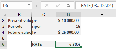
Required annual return to meet goal.

2. Pension Annuity Funding

Scenario:
$100,000 fund providing $750/month for 15 years (payments at start of month).

Calculation:

=RATE(15*12,-750,100000,,1)

Result: 0.3548% monthly (4.26% p.a.)

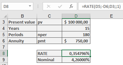
Required monthly compounding rate.

3. Mortgage Pricing

Scenario:
$175,000 loan with $1,000 monthly payments over 30 years.

Calculation:

=RATE(30*12,-1000,175000)

Result: 0.4632% monthly (5.56% p.a.)

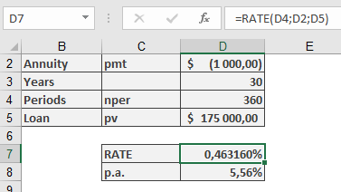
Effective annual interest rate.

Technical Notes

1. Iterative Process:
   • Begins with Guess value (default 10%)
   • Uses Newton-Raphson approximation
   • May fail to converge if no solution exists
2. Complementary Functions:
   • IRR(): For irregular cash flows
   • XIRR(): For irregular dates
   • NPER(): For term calculations
3. Financial Best Practices:
   • For monthly results, multiply by 12 for APR
   • Use negative values for cash outflows
   • Combine with ROUND() for presentation:

=ROUND(RATE(…)*12,2)& »% p.a. »

Its calculates the present value of an investment based on a constant interest rate and a series of future payments (annuities) and/or a lump sum.

Syntax

PV(Rate; Nper; [Pmt]; [Fv]; [Type])

Arguments

Argument	Requirement	Description	Financial Meaning
Rate	Required	Interest rate per period	Cost of capital/discount rate
Nper	Required	Total number of periods	Investment/loan term
[Pmt]	Conditionally Required	Payment per period	Annuity amount
[Fv]	Optional	Future value	Target balance/residual value
[Type]	Optional	Payment timing: 0 = end period (default) 1 = beginning period	Cash flow timing

Note: Either Pmt or Fv must be provided.

Financial Model

Implements the time value of money principle:

PV + Σ[Pmt/(1+Rate)^k] + Fv/(1+Rate)^Nper = 0

where k ranges from 1 to Nper (adjusted for Type).

Key Applications

1. Lump Sum Investments (Retirement Planning)

=PV(Rate, Nper,, Fv)

1. Annuity Valuation (Pension Planning)

=PV(Rate, Nper, Pmt)

1. Loan Capacity (Mortgage Underwriting)

=PV(Rate, Nper, -Pmt)

Examples

1. Retirement Savings Verification

Scenario:
$10,000 invested for 15 years at 5% p.a. targeting $25,000.

Calculation:

=PV(5%, 15,, 25000)

Result: -$12,025.43

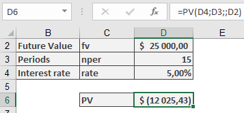
Interpretation: Requires $12,025 initial investment to reach target (current $10,000 insufficient).

2. Mortgage Qualification

Scenario:
$1,000 monthly payment capacity for 30 years at 5.5% p.a.

Calculation:

=PV(5.5%/12, 30*12, -1000)

Result: $176,121.76

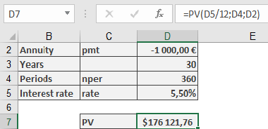
Interpretation: Maximum loan amount at given terms.

Important Notes

1. Sign Convention:
   • Positive results = Cash inflows
   • Negative results = Cash outflows
2. Compounding Assumptions:
   • For monthly payments, divide annual rate by 12
   • For quarterly payments, divide annual rate by 4
3. Precision Tip:
   For loan amortization schedules, combine with ROUND():

=ROUND(PV(…), 2)

Its calculates the price per 100 currency units of face value for a security that pays simple interest at maturity (no compounding).

Syntax

PRICEMAT(Settlement; Maturity; Issue; Rate; Yield; [Basis])

Arguments

Argument	Requirement	Description	Validation Rules
Settlement	Required	Trade date	Must be valid date < Maturity
maturity	Required	Maturity date	Must be valid date > Settlement
issue	Required	Security issuance date	Must be valid date ≤ Settlement
rate	Required	Annual coupon rate	≥ 0
yield	Required	Annual market yield	≥ 0
[basis]	Optional	Day count convention (0-4)	Default=0

Error Conditions

• #VALUE!: Invalid dates
• #NUM!: Negative rates/yields or Basis ∉ {0,1,2,3,4}

Key Features

1. Simple Interest Model:
   • Interest calculated linearly (no compounding)
   • Appropriate for short-term instruments
2. Price Components:
   • Principal repayment at maturity
   • Full-term interest payment
   • Discounted at market yield

Calculation Method

Price = [Repayment + (Rate × DIM/YearDays)] / (1 + Yield × DSM/YearDays) – Accrued Interest

Where:

• DIM = Days from issue to maturity
• DSM = Days from settlement to maturity
• YearDays = Days in year per Basis

Example

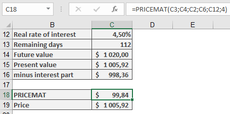
Important Notes

1. Day Count Conventions:
   • 0 = US (NASD) 30/360
   • 1 = Actual/actual
   • 2 = Actual/360
   • 3 = Actual/365
   • 4 = European 30/360
2. Financial Applications:
   • Commercial paper
   • Short-term notes
   • Certificates of deposit
3. Complementary Functions:
   • ACCRINT(): Calculates accrued interest
   • YIELDMAT(): Determines equivalent yield
4. Implementation Tip:
   For precise institutional calculations:

=ROUND(PRICEMAT(…),2) + ROUND(ACCRINT(…),2)