Catégorie : Excel function

This function returns the geometric mean of a set of positive numbers. The geometric mean is particularly useful for calculating average growth rates (e.g., compound interest, variable returns, or percentage-based trends).

The geometric mean is computed as the n-th root of the product of all values, where n is the number of values:​​

Syntax:

GEOMEAN(number1; [number2]; …)

Arguments:

• number1 (required) – The first number or range for calculation.
• number2, … (optional) – Additional numbers or ranges (up to 255 in modern Excel).
• Note: Arguments can be supplied as individual values, arrays, or cell references.

Background:

The geometric mean is ideal for analyzing percentage-based changes (e.g., growth rates, inflation, or multiplicative processes), where the arithmetic mean would produce misleading results.

Example:

Scenario:
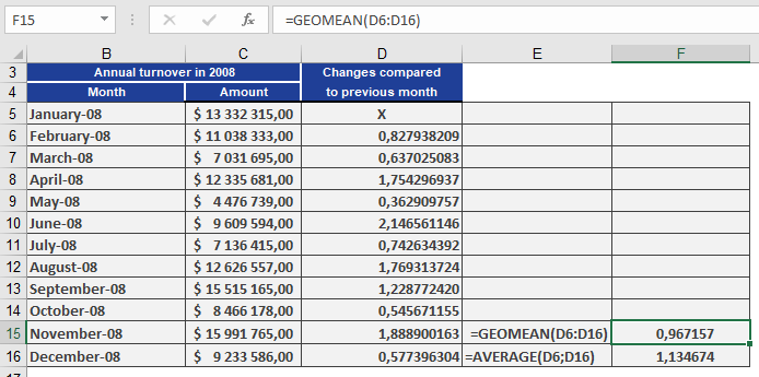
As a controlling manager at a software company, you want to determine the average monthly sales growth rate over a period.

Problem:

• Using the arithmetic mean would overestimate growth (e.g., showing 113% average growth).
• The geometric mean correctly reflects the compounded trend, revealing an average 97% growth factor (i.e., a 3% decline).

Steps:

1. Calculate monthly growth factors (current month / previous month).
2. Apply GEOMEAN() to these factors to derive the true average growth rate.

Result:
The geometric mean (97%) indicates a net decline, while the arithmetic mean (113%) falsely suggests growth.

Key Insight:

• Geometric mean = Accurate for multiplicative processes (e.g., finance, biology).
• Arithmetic mean = Misleading for volatile or percentage-based data.

This function returns the natural logarithm of the gamma function, Γ(x), calculated with 15-digit precision.

Syntax:

=GAMMALN.PRECISE(x)

Arguments:

• x (required) – The value for which you want to calculate GAMMALN.PRECISE().

Background:

For background details, refer to the documentation for the GAMMALN() function.

Example:

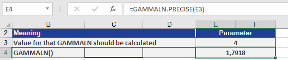
For usage examples demonstrating the GAMMALN.PRECISE functions below;

This function returns the natural logarithm of the gamma function, Γ(*x*).

Syntax:

GAMMALN(x)

Arguments:

• x (required) – The value for which you want to calculate GAMMALN().

Background:

The GAMMALN() function returns the natural logarithm (base *e*) of the gamma function.

A logarithm of a number is the exponent to which a fixed base must be raised to produce that number. Common logarithms include:

• Natural logarithm (ln): Base *e* (Euler’s number ≈ 2.71828)
• Base-10 logarithm (log₁₀)
• Base-2 logarithm (log₂)

The logarithm (to base *b*) of a number *y* is the exponent by which *b* must be raised to obtain *y*. Thus, the logarithmic function is the inverse of the exponential function.

Calculation:

GAMMALN(x) is computed as:

ln⁡(Γ(x))ln(Γ(x))

where Γ(x) is the gamma function.

Example:

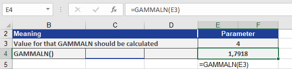
To calculate GAMMALN(4), refer to Figure below, which illustrates the computation.

The GAMMALN() function returns the natural logarithm 1.7918 for the gamma function evaluated at *x* = 4.

This function returns the probabilities of a gamma-distributed random variable. It is used to analyze variables with a skewed distribution, commonly applied in queuing theory and other statistical analyses.

Syntax

GAMMA.DIST(x; alpha; beta; cumulative)

Arguments

• x (required) – The value (quantile) for which the probability is calculated.
• alpha (required) – A shape parameter of the distribution.
• beta (required) – A scale parameter of the distribution. If beta = 1, the function returns the standard gamma distribution.
• cumulative (required) – A logical value determining the function type:
  • If TRUE, GAMMA.DIST() returns the cumulative distribution function (probability that a random event occurs between 0 and x).
  • If FALSE, it returns the probability density function.

Background

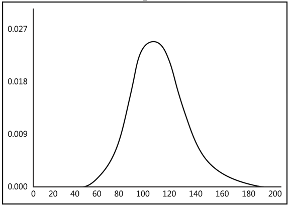
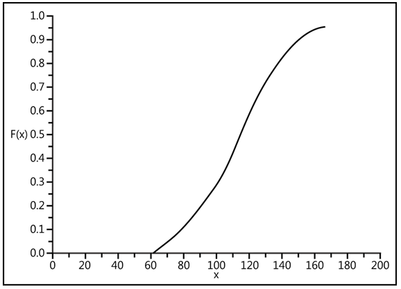
The gamma distribution is a continuous probability distribution for positive real numbers (see Figure below). Its probability density function is defined for x > 0, with f(x) = 0 for other values.

Key Properties:

• Parameters p (alpha) and q (beta) must be > 0.
• The prefactor bᵖ/Γ(p) ensures correct normalization, where Γ(p) is the gamma function.
• Expected value (mean) = αβ
• Variance = αβ²

Reproductive Property:

• If X and Y are independent gamma-distributed variables with parameters (β, pₓ) and (β, pᵧ), their sum X + Y follows a gamma distribution with parameters (β, pₓ + pᵧ).

Special Cases:

• The chi-square distribution (with k degrees of freedom) is a gamma distribution where p = k/2, β = ½.
• The exponential distribution (with rate λ) is a gamma distribution with p = 1, β = λ.
• The Erlang distribution (with λ and n degrees of freedom) corresponds to p = n, β = λ.
• The quotient X/(X + Y) of two independent gamma-distributed variables follows a beta distribution with parameters pₓ and pᵧ.

Parameterization Note:

• Some literature uses alternative parameterizations (e.g., αβ for mean). To avoid confusion, explicitly state moments (e.g., mean = αβ, variance = αβ²). See Figure below.

Function Details

• GAMMA.DIST() is a two-parameter (alpha, beta) mathematical distribution based on the gamma function.
• It is the inverse of GAMMA.INV().

Example

Calculate GAMMA.DIST() using the following inputs:

• x = 10 (quantile value)
• alpha = 2.70 (shape parameter)
• beta = 2 (scale parameter)

Results (see Figure below):

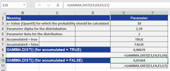
• 0.90679 (cumulative = TRUE)
• 0.03364 (cumulative = FALSE)

Key Takeaways

• The gamma distribution models skewed, positive continuous data.
• Parameters alpha (shape) and beta (scale) define its behavior.
• Cumulative = TRUE returns probabilities (CDF), while FALSE returns density values (PDF).
• Special cases include chi-square, exponential, and Erlang distributions.

This function is essential for advanced statistical modeling, particularly in reliability analysis and stochastic processes.

This function returns the quantile of the gamma distribution. If
p = GAMMA.DIST(x,…), then GAMMA.INV(p,…) = x.

Use this function to examine a variable whose distribution may be skewed.

Syntax:
GAMMA.INV(probability; alpha; beta)

Arguments:

• probability(required) – A probability associated with the gamma distribution.
• alpha(required) – A parameter of the distribution.
• beta(required) – A parameter of the distribution. If beta = 1, INV() returns the standard gamma distribution.

Background:
GAMMA.INV() is the inverse function of GAMMA.DIST() and can be used to model a gamma distribution. The alpha and beta arguments correspond to the values for the GAMMA.DIST() function. The probability can be any value from 0 through 100 percent. GAMMA.INV() calculates the position of x on the horizontal axis that matches the cumulative area ratio of the gamma distribution.

Example:
Use the values in Figure below to calculate GAMMA.INV(). The figure also shows the calculation of GAMMA.INV().

The GAMMA.INV() function returns the quantile 10 for the gamma distribution based on the parameters shown.

This function returns a frequency distribution as a single-column matrix. For example, use FREQUENCY() to count sales within a specific range. Since FREQUENCY() returns an array of values, it must be entered as an array formula.

Syntax

FREQUENCY(data_array; bins_array)

Arguments

• data_array (required) – An array of or reference to a set of values for which you want to count frequencies. If data_array contains no values, FREQUENCY() returns an array of zeros.
• bins_array (required) – An array of or reference to intervals used to group the values in data_array. If bins_array contains no values, FREQUENCY() returns the number of elements in data_array.

Background

To simplify quantitative data analysis, values are categorized into classes, and their frequencies are calculated. Keep the following in mind:

• Too many classes provide more detail but reduce overall clarity, while too few classes oversimplify the data.
• Classes do not need to be of equal size.

Unlike the COUNTIF() function, FREQUENCY() does not require manual entry in each result cell. Instead, it can be entered once as an array formula, returning results across multiple cells.

Example

We’ll use the example of a software company’s sales data. A sales representative recorded monthly sales over two years in Excel. The manager wants sales categorized as:

• Up to $15,000
• Up to $17,000
• Up to $19,000
• More than $19,000

Thus, four classes are needed.

• The data to be classified is in cells C3:C26 (see Figure below).
• The class intervals are defined in the Class column.
• The frequency of data within each class is calculated based on these intervals.

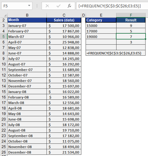
Since FREQUENCY() is an array function, select all four result cells (F3:F6) to display the output as an array.

The FORECAST() function predicts a future value (y) based on existing linear trends in your data. It uses linear regression to estimate the dependent variable (y) for a given independent variable (x).

Syntax

FORECAST(x; known_y’s; known_x’s)

When to Use

• Predict future sales, inventory needs, or consumer trends.
• Estimate values along a linear trendline.

Arguments

Argument	Required	Description
x	Yes	The data point (independent variable) for which you want to predict a value.
known_y’s	Yes	The dependent data range (values you want to predict, e.g., sales numbers).
known_x’s	Yes	The independent data range (e.g., time periods, ad spend).

Background

How It Works

1. Fits a linear trend (y = mx + b) to your historical data (known_x’s, known_y’s).
2. Predicts y for a new x value along this trendline.

Limitations

• Assumes a linear relationship between x and y.
• For non-linear trends, use GROWTH() (exponential) or TREND() (array-based).

Example: Predicting Website Visits & Online Orders

Scenario

As a marketing director, you want to forecast:

1. Online orders based on predicted visits.

Forecast Online Orders

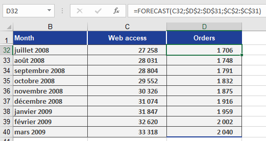
• x: Predicted visits (C32).
• known_y’s: D2:D31 (Orders from Jan 2005 – Jun 2008).
• known_x’s: C2:C31 (Historical visits).

Formula:

=FORECAST(C32, D2:D31, C2:C31)

Result: Predicts orders for July 2008 (Figure below).

Copying the Formula

Use absolute references (e.g., $C$2:$C$31) to drag the formula across cells D33:D40 for future months.

Key Takeaways

 Best for Linear Trends: Simple, fast predictions when data follows a straight-line pattern.
 Not for Complex Trends: Use TREND() or GROWTH() for non-linear data.
 Workflow:

1. Organize historical x and y data.
2. Apply FORECAST(x, known_y’s, known_x’s).
3. Copy formulas for multiple predictions.

The FISHERINV() function reverts a Fisher-transformed value (y) back to its original correlation coefficient (x). It is the inverse of the FISHER() function, ensuring that:

• If y = FISHER(x), then FISHERINV(y) = x.

Syntax

FISHERINV(y)

Arguments

• y (required): A numeric value representing a Fisher-transformed (z) value that you want to convert back to a correlation coefficient.

Background

Purpose

• Reverses the Fisher Transformation: Converts a normally distributed z-value (from FISHER()) back to a correlation coefficient (r).
• Critical for Averaging Correlations: After averaging Fisher-transformed values, FISHERINV() restores the result to the interpretable -1 to +1 scale.

Mathematical Formula

The inverse Fisher transformation is calculated as:

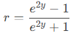
Where:

• y = Fisher-transformed (z) value.
• r = Original correlation coefficient.

Example

Context

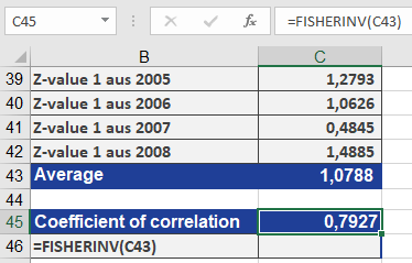
Referencing the FISHER() example:

1. Transformed yearly correlation coefficients (r) into z-values using FISHER().
2. Averaged the z-values.
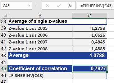
3. Applied FISHERINV() to revert the averaged z back to a single r (result: 0.7927).

Why This Matters

• Ensures valid interpretation of averaged correlations.
• Preserves the mathematical properties of correlation coefficients.

Key Takeaways

• Use Case: Revert Fisher-transformed data (z) to original correlations (r).
• Pair with FISHER(): Essential for averaging correlations or hypothesis testing.
• Output Range: Returns values between -1 and 1 (standard correlation scale).

Visual Workflow

1. Original r → FISHER(r) → z (normalized).
2. Average z-values.
3. FISHERINV(z_avg) → Final r (interpretable result).

The FISHER() function computes the Fisher transformation of a given value x. This transformation converts a correlation coefficient (which ranges between -1 and +1) into an approximately normally distributed variable, enabling statistical tests on correlation data.

Syntax

FISHER(x)

Arguments

• x (required): A numeric value between -1 and 1 (typically a correlation coefficient r) that you want to transform.

Background

Correlation vs. Regression

• Correlation (r) measures the linear relationship between two variables.
  • Ranges from -1 (perfect negative correlation) to +1 (perfect positive correlation).
  • 0 indicates no linear relationship.
• Regression describes how one variable predicts another, while correlation quantifies their association.

Why Use Fisher Transformation?

1. Non-Interval Scaling:
   • The difference between r=0.2 and r=0.4 is not equivalent to the difference between r=0.4 and r=0.6.
   • Direct averaging of correlation coefficients is invalid.
2. Normalization:
   • The Fisher z-transformation converts skewed correlation data into a normal distribution, allowing:
     • Hypothesis testing (e.g., « Is the correlation significant? »).
     • Averaging multiple correlations.

Formula

The Fisher transformation is calculated as:

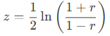
Where:

• r = Correlation coefficient.
• z = Transformed (normally distributed) value.

Steps to Average Correlations

1. Transform each r to z using FISHER().
2. Average the z-values.
3. Revert the averaged z back to r using FISHERINV().

Example: Website Visits vs. Online Orders

Scenario

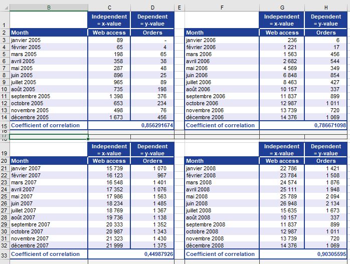
A software company (founded in 2005) analyzes website visits and online orders (2019–2022) to determine if marketing efforts (e.g., newsletters) drive sales.

Data

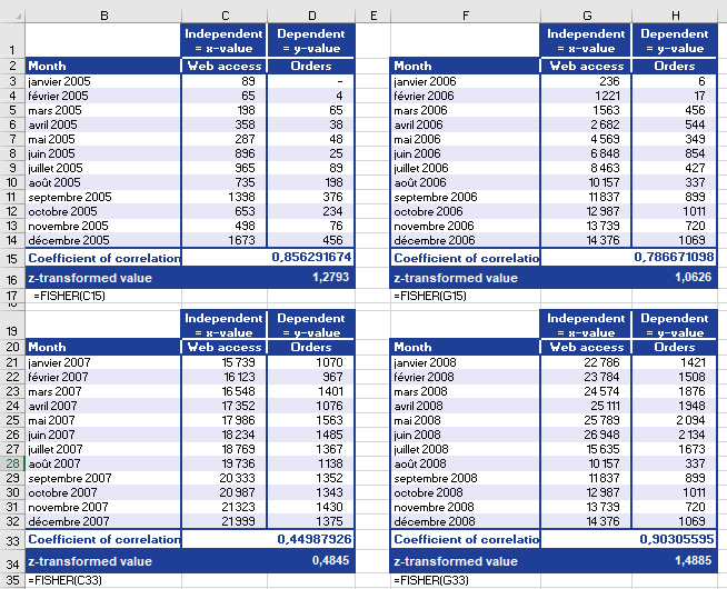
• Yearly correlation coefficients (r) between visits and orders (Figure below).
• Problem: Cannot directly average r values (non-interval scaled).

Solution

1. Transform r to z
   • Use FISHER(r) for each year (Figure below).

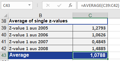
1. Average z-values (Figure below).

1. Revert to r
   • Apply FISHERINV(z_avg) → Final r = 0.7927 (Figure below).

Interpretation

• r = 0.7927: Strong positive correlation.
  • As website visits ↑, online orders ↑.
• Conclusion: Marketing-driven visits significantly increase orders.

Key Takeaways

• Use FISHER() to:
  • Normalize correlation data for statistical tests.
  • Compute averages of multiple correlations.
• Use FISHERINV() to revert z back to r.
• Limitation: Only valid for -1 < r < 1.

This function returns the test statistic of an F-test, which calculates the one-tailed probability that the variances of two datasets (array1 and array2) are not significantly different.

Syntax

F.TEST(array1; array2)

Arguments

• array1 (required): The first dataset (range or array).
• array2 (required): The second dataset (range or array).

Background

The F.TEST() function determines whether two samples exhibit different variances. For example:

• Compare test scores from public vs. private schools to assess differences in score variability.
• Evaluate whether the variance between two groups is statistically significant.

Key Notes:

1. Purpose: Tests if two sample variances are equal.
2. Output: Returns a significance level (p-value) between 0 and 1 (or 0%–100%).
   • A high p-value (e.g., 0.89) suggests no significant difference in variances.
   • A low p-value (e.g., <0.05) indicates significant differences.
3. Calculation: Directly computes significance from raw data without pre-calculating variances.

Example: Clinical Drug Study

Scenario

• Goal: Test if an increased drug dosage speeds up recovery.
• Groups:
  • Control group: Standard daily dosage.
  • Test group: Higher initial dosage.
• Metric: Treatment duration (days).

Hypotheses

• Null (H₀): No difference in treatment efficacy.
• Alternative (H₁): Higher dosage improves recovery time.

Analysis

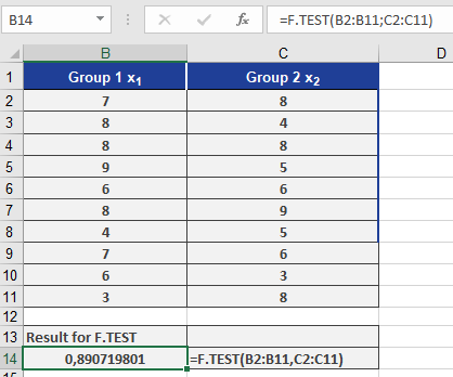
1. F.TEST Result: 0.89 (89%) (see Figure below).

1. • Interpretation: 89% probability that variance differences are due to chance.
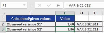
2. Variance Comparison (Figure below):
   • Minor differences between groups.
   • Confirms H₀ (no significant variance difference).

Conclusion

• Retain H₀: No evidence that higher dosage alters recovery time variability.

Key Takeaways

• Use F.TEST() to compare variances of two datasets.
• High p-value (e.g., >0.05): Fail to reject H₀ (variances are similar).
• Low p-value (e.g., ≤0.05): Reject H₀ (significant variance difference).