Votre panier est actuellement vide !
Catégorie : Excel function
How to use the MAX() function in Excel
This function returns the largest value from a set of arguments.
Syntax:
MAX(number1; [number2]; …)Arguments:
- number1 (required): First number, cell reference, or range to evaluate
- number2,… (optional): Additional numbers, references, or ranges
Key Features:
- Data Handling:
- Accepts numbers, empty cells, logical values (TRUE/FALSE), and text representations of numbers
- Ignores text values that cannot be converted to numbers
- Returns 0 if no numbers are found in the arguments
- Range Behavior:
- When evaluating ranges or arrays:
✓ Processes only numerical values
✓ Automatically ignores empty cells, text, and logical values - To include logical values and text numbers, use MAXA()
- When evaluating ranges or arrays:
- Error Handling:
- Returns errors if any argument contains unprocessable text or error values
Comparison:
- For minimum values, use MIN() with identical argument rules
- For more inclusive calculations, use MAXA()/MINA()
Example:
As Accounting Manager, you need to find the highest sales figure from two years of unsorted data (see Figure below).Implementation:
=MAX(C3:C26)
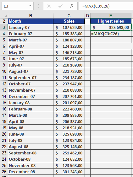
This formula will return the single highest value from cells C3 through C26, regardless of their position in the range.
Note: The function is particularly useful for:
- Identifying performance outliers
- Finding threshold values
- Data validation checks
How to use the LOGNORM.DIST() function in Excel
This function returns values from the lognormal distribution where the natural logarithm of the random variable follows a normal distribution with parameters μ (mean) and σ (standard_dev). The probability density function (PDF) is given by:

Syntax
LOGNORM.DIST(x; mean; standard_dev; cumulative)
Arguments
- x (required): Evaluation point (x>0x>0)
- mean (required): Mean of ln(x)ln(x) (μμ)
- standard_dev (required): Standard deviation of ln(x)ln(x) (σ>0σ>0)
- cumulative (required):
- TRUE: Returns cumulative distribution (CDF):
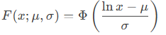
where ΦΦ is the standard normal CDF.
-
- FALSE: Returns probability density (PDF)
Background
The lognormal distribution models multiplicative processes where:
- Skewness: Right-tailed distribution
- Multiplicative effects: If X=eYX=eY with Y∼N(μ,σ2)Y∼N(μ,σ2), then XX is lognormal
- Real-world examples:
- Income distributions (growth rates compound multiplicatively)
- Particle sizes in aerosols
Key properties:
- Mean: eμ+σ2/2eμ+σ2/2
- Variance: (eσ2−1)e2μ+σ2(eσ2−1)e2μ+σ2
Example Calculation
Given:
- x=4x=4
- μ=3.5μ=3.5
- σ=1.2σ=1.2
- Cumulative = TRUE
Compute F(4;3.5,1.2):
- Standardize: z=ln(4)−3.51.2≈−0.747z=1.2ln(4)−3.5≈−0.747
- Evaluate Φ(−0.747)≈0.039084Φ(−0.747)≈0.039084
Result:
LOGNORM.DIST(4, 3.5, 1.2, TRUE) = 0.039084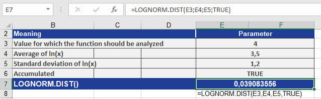
How to use the LOGNORM.INV() function in Excel
This function returns the quantile (inverse cumulative distribution) of a lognormal distribution, where the natural logarithm of the random variable *x* is normally distributed with specified mean and standard deviation parameters.
If:
p = LOGNORM.DIST(x, mean, standard_dev, TRUE)
Then:
x = LOGNORM.INV(p, mean, standard_dev)This means that for a given probability *p*, you can calculate the corresponding quantile value *x* from the lognormal distribution. Use this function to work with data that has been logarithmically transformed.
Syntax:
LOGNORM.INV(probability; mean; standard_dev)Arguments:
- probability (required): The probability value (0 ≤ *p* ≤ 1) associated with the lognormal distribution.
- mean (required): The mean (μ) of the natural logarithm of *x* (i.e., the mean of ln(*x*)).
- standard_dev (required): The standard deviation (σ) of the natural logarithm of *x* (i.e., the standard deviation of ln(*x*)).
Background:
The inverse lognormal distribution function calculates the value *x* such that the cumulative probability up to *x* equals the specified probability *p*. Mathematically, it is expressed as: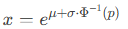
where:
- Φ−1(p)Φ−1(p) is the inverse of the standard normal cumulative distribution function (quantile function of the normal distribution).
- *e* is the base of the natural logarithm (~2.71828).
Example:
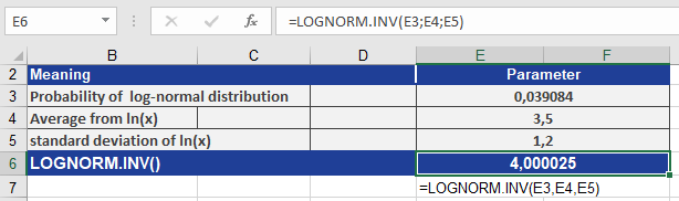
Calculate LOGNORM.INV() using the following inputs:- probability = 0.039084 (the cumulative probability associated with the lognormal distribution)
- mean = 3.5 (the mean of ln(*x*))
- standard_dev = 1.2 (the standard deviation of ln(*x*))
The calculation is illustrated in Figure below.
Result:
The function returns the quantile value 4.000025, meaning that there is a 3.9084% probability that a value from this lognormal distribution will be less than or equal to 4.000025.How to use the LOGEST() function in Excel
This function calculates the exponential curve in regression analyses and returns an array of values describing this curve. Since it returns an array, it must be entered as an array formula.
Syntax:
LOGEST(known_y’s, known_x’s, const, stats)Arguments:
- known_y’s(required): The known y-values from the relationship y = b * m^x.
- If known_y’sis a single column, each column in known_x’s is treated as a separate variable.
- If known_y’sis a single row, each row in known_x’s is treated as a separate variable.
- known_x’s(optional): The known x-values from the relationship y = b * m^x.
- The known_x’sarray can include one or more sets of variables. If only one variable is used, known_y’s and known_x’s can be ranges of any shape as long as they have equal dimensions. If multiple variables are used, known_y’s must be a single row or column (a vector).
- If known_x’sis omitted, it defaults to {1,2,3,…} with the same number of elements as known_y’s.
- const(optional): A logical value determining whether to force the constant b to equal 1.
- If constis TRUE or omitted, b is calculated normally.
- If constis FALSE, b is set to 1, and the m-values are adjusted so that y = m^x.
- stats(optional): A logical value specifying whether to return additional regression statistics.
- If statsis TRUE, LOGEST() returns additional statistics in the array format:
{mn, mn-1, …, m1, b; sen, sen-1, …, se1, seb; r², sey; F, df, ssreg, ssresid} - If statsis FALSE or omitted, LOGEST() returns only the m-coefficients and constant b.
- If statsis TRUE, LOGEST() returns additional statistics in the array format:
Background:
Unlike LINEST(), which fits a straight line, LOGEST() describes the relationship between dependent y-values and independent x-values using an exponential curve of the form:
y = b × m^xHere, y and x can be vectors. Each base m has an associated exponent x, meaning references or values must have the same number of elements.
If only one independent x-variable exists, you can calculate:
- Slope (m): =INDEX(LOGEST(known_y’s, known_x’s), 1)
- y-intercept (b): =INDEX(LOGEST(known_y’s, known_x’s), 2)
Use the equation y = b * m^x to predict future y-values. Alternatively, the GROWTH() function can be used for estimation.
When using an array constant (e.g., values_x) as an argument, separate row values with commas and column values with semicolons.
Example:
To illustrate regression value calculations, consider the example used for LINEST(). A company observed a significant increase in online orders and wants to determine whether this growth correlates with website visits.The marketing department analyzes past 18 months of data, comparing website visits to online orders using LOGEST() (see Figure below).
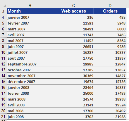
A chart (Figure below) shows that orders exhibit exponential growth relative to website visits, suggesting a strong correlation.

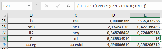
Using LOGEST(), the regression results are computed and displayed in Figure below.
- known_y’s(required): The known y-values from the relationship y = b * m^x.
How to use the LARGE() function in Excel
This function returns the k-th largest value in a data set. Use this function to select a value based on its relative size. For example, you can use LARGE() to calculate the top three sales in a table.
Syntax: LARGE(array, k)
Arguments
- array (required): The array or range of data for which you want to determine the k-th largest value.
- k (required): The position of the element in the array or cell range to return (e.g., 1 for the largest value, 2 for the second-largest, etc.).
Background
The MIN() and MAX() functions find the smallest or largest value in a range, but if you need the second-largest or third-smallest value, use LARGE() and SMALL().
- LARGE() returns the largest values.
- SMALL() returns the smallest values from a range.
Notes
- If array is empty, LARGE() returns the #NUM! error.
- If k is ≤ 0 or greater than the number of data points, the function returns #NUM!.
- If n is the number of data points in a range:
- LARGE(array, 1) returns the largest value.
- LARGE(array, n) returns the smallest value.
Examples
Software Company Example
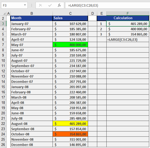
Assume a software company has a table with sales from the last two years and wants to find the three highest sales without sorting the data. The LARGE() function retrieves the three largest values, as shown in Figure below.
How to use the KURT() function in Excel
Returns the kurtosis of a dataset, which measures the « tailedness » and peakedness of a distribution compared to a normal distribution.
Syntax:
KURT(number1; [number2]; …)Arguments
Argument Required? Description number1 Yes First data point or range. number2, … Optional Additional data points Notes:
- Accepts arrays or cell ranges (e.g., A1:A10).
- Requires at least 4 data points; otherwise, returns #DIV/0!.
Background
Kurtosis Types:
- Mesokurtic (kurtosis = 0): Matches a normal distribution.
- Leptokurtic (kurtosis > 0): Sharper peak, heavier tails (e.g., financial returns).
- Platykurtic (kurtosis < 0): Flatter peak, thinner tails (e.g., uniform distribution).
Formula:
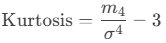
Where:
- m4m4: Fourth central moment.
- σσ: Standard deviation.
- Subtracting 3 adjusts for comparison to a normal distribution (excess kurtosis).
Example: Website Click Analysis
Scenario:
A software company evaluates click distributions:- Download Area: Kurtosis = –1.27 (platykurtic).
- Entire Website: Kurtosis = 0.42 (leptokurtic).

Interpretation:
Distribution Kurtosis Shape Implication Download Area –1.27 Flatter than normal Clicks are more spread out, fewer extreme values. Entire Website 0.42 Peaked with heavier tails Clicks cluster around the mean, with more outliers. Key Takeaways
- High Kurtosis (>0):
- Sharp peak, frequent outliers.
- Common in financial data (e.g., stock market crashes).
- Low Kurtosis (<0):
- Broad peak, fewer outliers.
- Seen in uniform distributions (e.g., dice rolls).
- Use Cases:
- Risk assessment (finance).
- Quality control (manufacturing).
Excel Tip: Combine with SKEW() to fully describe distribution shape.
How to use the INTERCEPT() function in Excel
Calculates the y-intercept of the linear regression line fitted to a dataset. This is the point where the regression line crosses the y-axis (i.e., the predicted value of y when x = 0).
Syntax:
INTERCEPT(known_y’s; known_x’s)Arguments
Argument Required? Description known_y’s Yes Dependent variable (response data). Must be a single row/column. known_x’s Yes Independent variable (predictor data). Must match dimensions of known_y’s. Error Handling:
- Returns #N/A if:
- known_y’s and known_x’s have unequal lengths.
- Either argument is empty.
Background
Regression Analysis Context:
- Models the linear relationship between dependent (y) and independent (x) variables.
- The regression line minimizes the sum of squared deviations (least squares method).
Equation of the Line:
y=mx+b
Where:
- b= y-intercept (calculated by INTERCEPT()).
- m = slope (calculated by SLOPE()).
Intercept Formula:
b=yˉ−mxˉ
- yˉ: Mean of known_y’s.
- xˉ: Mean of known_x’s.
Example: Website Traffic Analysis
Scenario:
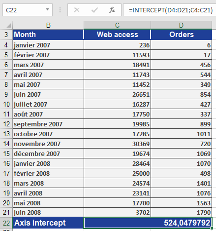
A company analyzes if orders (y) depend on website visits (x) (Jan 2007–Jun 2008).Step 1: Calculate Intercept
=INTERCEPT(orders_range ; visits_range)
Result: 524.05 (see Figure below).
Step 2: Interpret Results
- The intercept (b = 524.05) implies:
- If there are zero visits, the model predicts 524 orders (theoretical baseline).
- Combined with the slope (m), it defines the regression line equation.
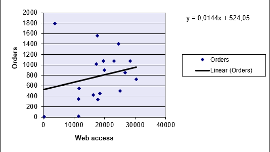
Visualization:
- A scatter plot with a trendline shows the intercept at y = 524.05 (Figure below).
Key Notes
- Usage with SLOPE():
- Use both functions to fully define the regression line:
y = SLOPE(y’s, x’s) * x + INTERCEPT(y’s, x’s)
- Assumptions:
- Linear relationship between x and y.
- Homoscedasticity (constant variance of residuals).
- Practical Applications:
- Forecasting sales based on advertising spend.
- Predicting exam scores from study hours.
- Returns #N/A if:
How to use the HYPGEOM.DIST() function in Excel
This function returns probabilities for a hypergeometrically distributed random variable. It calculates the probability of obtaining a specific number of successes in a sample drawn from a finite population without replacement.
Syntax:
HYPGEOM.DIST(sample_s; number_sample; population_s; number_population; cumulative)Required Information:
- Number of successes in the sample
- Size of the sample
- Number of possible successes in the population
- Size of the population
- Logical value determining the function type
Arguments
- sample_s (required): The number of successes in the sample.
- number_sample (required): The size of the sample.
- population_s (required): The number of successes in the population.
- number_population (required): The total size of the population.
- cumulative (required): A logical value that determines the function form:
- FALSE: Returns the probability mass function (exact probability).
- TRUE: Returns the cumulative distribution function.
Background
The hypergeometric distribution answers: « What is the probability of finding x successes in a sample drawn from a finite population? »
Key Characteristics:
- Used when sampling without replacement from a finite population.
- Each observation is either a success or failure.
- Subsets are chosen with equal likelihood.
Equation:
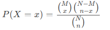
Where:
- x=sample_s
- n=number_sample
- M=population_s
- N=number_population
Example: Lottery Probability
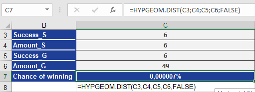
Scenario: Calculate the probability of winning a lottery with 6 numbers drawn from 49.
Arguments:
- sample_s = 6 (winning numbers in ticket)
- number_sample = 6 (numbers drawn)
- population_s = 6 (total winning numbers)
- number_population = 49 (total balls)
- cumulative = FALSE (exact probability)
Calculations:
- Probability of 6/6 (Jackpot):
=HYPGEOM.DIST(6, 6, 6, 49, FALSE) → 0.00000715% (Figure below).
- Probabilities for Smaller Wins:
- 5/6: =HYPGEOM.DIST(5, 6, 6, 49, FALSE) → 0.0018%
- 4/6: =HYPGEOM.DIST(4, 6, 6, 49, FALSE) → 0.10%
- 3/6: =HYPGEOM.DIST(3, 6, 6, 49, FALSE) → 1.77% (Figure below).

Conclusion:
The hypergeometric distribution precisely models scenarios with finite populations and without replacement, such as lotteries or quality control testing.How to use the HARMEAN() function in Excel
Returns the harmonic mean of a dataset, which is the reciprocal of the arithmetic average of reciprocals.
Syntax:
HARMEAN(number1; [number2]; …)Arguments
- number1 (required) – First value or range for calculation.
- number2, … (optional) – Additional values or ranges.
- Can use a single array (e.g., A1:A5) instead of comma-separated values.
Background
The harmonic mean is used for:
- Averaging rates or ratios (e.g., speed = distance/time).
- Cases where values are defined by reciprocal relationships.
Equation:
Harmonic Mean=n1x1+1×2+⋯+1xnHarmonic Mean=x11+x21+⋯+xn1n

where n = number of values, x = data points.
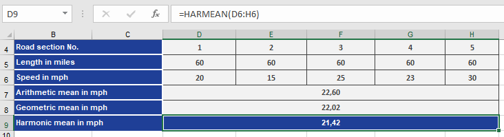
Example. To explain how the harmonic mean is calculated, use the previously mentioned example of speed and time. A bicyclist travels 300
miles through the Alps. The distance is divided into five legs, for which he measures the speed of each.
Now the bicyclist wants to calculate the average speed from the speeds reached in each leg. The result should show the consistent speed at which he could have traveled the same distance in the same time (see Figure below).
To get a better overview, he also calculated the arithmetic average and the geometric mean.
To find out what calculation returns the best result, he transforms the results of the arithmetic, geometric, and harmonic means in meters/seconds and then calculates the time it would take to travel the 300 miles at the average speed (see figure below).
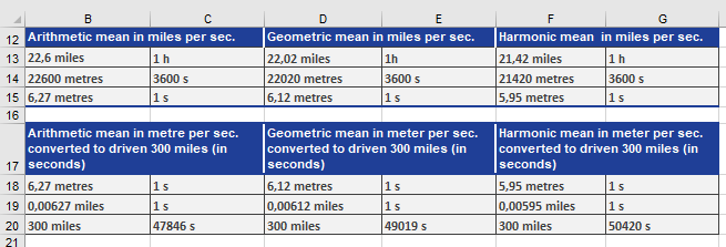
This calculation also confirms that the geometric mean is smaller than the harmonic mean, and the arithmetic mean is smaller than the geometric mean.
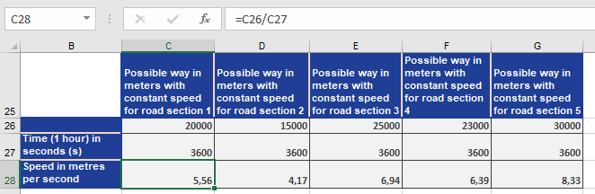
Next, you prove that the harmonic mean returns the best result. First you have to calculate speed v in m/s for the actual miles travelled at speed v for each leg in an hour. At a steady speed, the cyclist could have traveled 20 miles per hour in the first leg. If you divide 20 miles by 3,600 seconds, you get the speed v (see figure below).
Where V=S/t
Then you use the result for the speed in m/s in the same formula for t (time) to calculate the time for each leg in seconds. Given the fomular
t=S/V
the figure below shows the result.
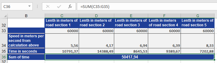
The sum of the times in seconds for the legs shows that the value is approximately the same as the harmonic mean. The difference of three seconds is based on the rounded values.
The comparison of the actual result of 50,417.94 seconds with the calculated results of the different means shows that the harmonic mean returns the best result.
Conclusion: The harmonic mean gives the most accurate average for rates.
How to use the GROWTH() function in Excel
The GROWTH function calculates predicted values based on an exponential trend. It returns y-values corresponding to a specified set of new x-values using existing x and y data. It can also fit an exponential curve to known data points.
Syntax:
GROWTH(known_y’s; known_x’s; new_x’s; const)Arguments
- known_y’s (required) – The dependent y-values from the exponential relationship y = b * m^x.
- If known_y’s is a single column, each column in known_x’s is treated as an independent variable.
- If known_y’s is a single row, each row in known_x’s is treated as an independent variable.
- known_x’s (optional) – The independent x-values from the relationship y = b * m^x.
- Supports single or multiple variable sets. If only one variable is used, known_y’s and known_x’s can be any shape but must have matching dimensions. For multiple variables, known_y’s must be a vector (single row or column).
- If omitted, defaults to {1, 2, 3, …} with the same length as known_y’s.
- Requirements:
- known_y’s and known_x’s must have the same number of rows/columns. A mismatch returns #REF!.
- Any zero or negative y-value returns #NUM!.
- new_x’s (optional) – New x-values for which to predict y-values.
- Must match known_x’s in structure:
- If known_y’s is a column, new_x’s must have the same columns.
- If known_y’s is a row, new_x’s must have the same rows.
- If omitted, defaults to known_x’s.
- If both known_x’s and new_x’s are omitted, they default to {1, 2, 3, …} (same length as known_y’s).
- Must match known_x’s in structure:
- const (optional) – Logical value controlling the constant b in y = b * m^x:
- TRUE (or omitted): Calculates b normally.
- FALSE: Forces b = 1, adjusting m to fit y = m^x.
Background
While TREND() models linear trends, GROWTH() fits exponential trends, useful when data grows by a fixed factor or percentage. It projects future values by fitting an exponential curve to historical data.
Example
A marketing manager analyzes website visits and online orders (Figure below), which grew exponentially from January 2007–June 2008. To forecast July 2008–March 2009:
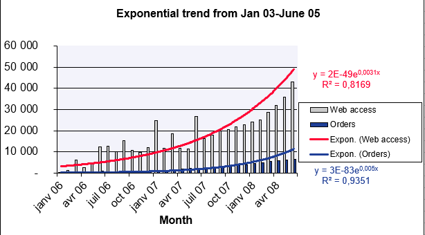
Website Visits Forecast
- known_y’s: Visits (Jan–Jun 2008).
- known_x’s: Months (Jan 2006–Jun 2008).
- new_x’s: Months (Jul 2008–Mar 2009).
- const: TRUE (calculate b normally).
Result: Predicted values shown in Figure below.
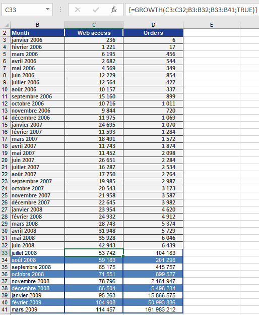
Online Orders Forecast
Using the same method, orders are projected (Figure below).

Conclusion
GROWTH() provides accurate exponential trend forecasts, assuming historical growth patterns continue.
- known_y’s (required) – The dependent y-values from the exponential relationship y = b * m^x.