Catégorie : Excel function

Its rounds a number to the nearest specified multiple, using standard rounding rules (up if remainder ≥ half of multiple).

Syntax

MROUND(number; multiple)

Arguments

Parameter	Requirement	Valid Input
number	Required	Numeric value to round
multiple	Required	Positive numeric value (rounding interval)

Key Properties

1. Rounding Rules:
   • Round Up if remainder ≥ multiple/2
   • Round Down if remainder < multiple/2
   • Follows banker’s rounding (toward nearest even for exact halves).
2. Error Handling:
   • #NUM! if number and multiple have opposite signs.
3. Special Cases:
   • If multiple = 0, returns 0.
   • If number = 0, returns 0 regardless of multiple.

Examples

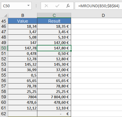
Comparison with Other Rounding Functions

Function	Behavior	Example (number=3.25, multiple=0.5)
MROUND()	Nearest multiple	3.5
CEILING()	Always up	3.5
FLOOR()	Always down	3.0
ROUND()	Nearest digit	3.2 (if rounding to 1 decimal)

Applications

• Pricing Strategies: Ensure prices end in 0.99 or 0.49.
• Manufacturing: Round measurements to standard units (e.g., 1/8″).
• Scheduling: Align timestamps to 5/10/15-minute blocks.

Error Handling

Error	Cause	Solution
#NUM!	number and multiple have opposite signs	Use same signs
#VALUE!	Non-numeric input	Validate data

 

The MOD returns the remainder after division of number by divisor, preserving the sign of the divisor.

Syntax

MOD(number; divisor)

Arguments

Parameter	Requirement	Valid Input
number	Required	Any real number (dividend)
divisor	Required	Non-zero real number

Key Properties

1. Mathematical Definition:

1. • Sign Rule: Result carries the sign of divisor.
   • Special Case: MOD(n, 1) returns the decimal part of n.
2. Error Handling:
   • #DIV/0! if divisor = 0.
3. Behavior for Negatives:

Example	Result	Explanation
=MOD(7,3)	1	Standard case
=MOD(-7,3)	2	Follows divisor’s sign (+)
=MOD(7,-3)	-2	Follows divisor’s sign (–)
=MOD(-7,-3)	-1	Follows divisor’s sign (–)

Examples

The MOD() function is often used together with other functions; for example, to add every second line (see Figure below).

The formula is {=SUM(IF(MOD(ROW(C3:C8);2)=0;C3:C8;0))}. Because this is an array formula, you have to press Ctrl+Page Up+Enter after you enter the formula.

Comparison with Other Methods

Method	Formula	-7 mod 3	Sign Rule
Excel MOD	n – d*INT(n/d)	2	Matches divisor
Symmetrical	n – d*TRUNC(n/d)	-1	Matches dividend

Applications

• Alternate Row Shading:

=MOD(ROW(),2)=0 → Conditional formatting rule 

• Time Calculations: Convert seconds to HH:MM:SS.
• Circular Buffers: Index wrapping in programming.

Its returns the matrix product of two arrays. The resulting matrix has:

• Rows = Number of rows in array1
• Columns = Number of columns in array2

Syntax

MMULT(array1; array2)

Arguments

Parameter	Requirement	Valid Input
array1	Required	Numeric array with dimensions m×n
array2	Required	Numeric array with dimensions n×p

Note: The number of columns in array1 must equal the number of rows in array2.

Key Properties

1. Mathematical Operation:
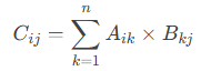
   For matrices A (m×n) and B (n×p), the product C (m×p) is calculated as:​

1. Input Rules:
   • Supports:
     • Cell ranges (e.g., A1:B2)
     • Array constants (e.g., {1,2;3,4})
     • Named ranges
   • Rejects:
     • Non-numeric/text → #VALUE!
     • Dimension mismatch → #VALUE!
2. Array Formula:
   • In legacy Excel, enter with Ctrl+Shift+Enter.
   • Excel 365 handles dynamic arrays automatically.

Examples

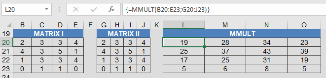
Real-World Use:

1. • Physics: Transformations in 3D space.
   • Finance: Portfolio risk calculations.
   • Engineering: Stress-strain models.

Why This Matters

• Solves systems of linear equations (e.g., with MINVERSE).
• Fundamental in computer graphics (rotation/scaling).
• Used in machine learning (neural networks).

Error Handling

Error	Cause	Solution
#VALUE!	Dimension mismatch/non-numeric input	Verify matrix dimensions

Related Functions

• MINVERSE(): Matrix inversion (for solving equations).
• MDETERM(): Matrix determinant (invertibility check).
• SUMPRODUCT(): Dot product for vectors.

Its returns the inverse of a square matrix if it exists (i.e., the matrix is non-singular).

Syntax

MINVERSE(array)

Argument

Parameter	Requirement	Valid Input
array	Required	Square numeric array (e.g., 2×2, 3×3)

Key Properties

1. Prerequisites:
   • Matrix must be square (equal rows/columns).
   • Determinant ≠ 0 (check with MDETERM()).
   • Rejects:
     • Non-numeric/text → #VALUE!
     • Non-square arrays → #VALUE!
     • Singular matrices → #NUM!
2. Mathematical Definition:
   For matrix A, its inverse A⁻¹ satisfies:

1. • Calculated via LU decomposition in Excel (16-digit precision).
2. Critical Notes:
   • Array Formula: Must be entered with Ctrl+Shift+Enter (legacy Excel) or Enter (dynamic arrays in Excel 365).
   • Numerical Stability: Rounding errors may occur for ill-conditioned matrices.

 Example

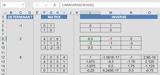
Why This Matters

• Engineering: Circuit analysis, structural modeling.
• Economics: Input-output models (Leontief).
• Computer Science: 3D transformations, cryptography.

Error Handling

Error	Cause	Solution
#VALUE!	Non-square/non-numeric input	Validate matrix dimensions/contents
#NUM!	Singular matrix (det=0)	Use pseudoinverse or reformulate problem

 

This function returns the determinant of a square matrix (array). The determinant is a scalar value that encodes key properties of the matrix, such as invertibility.

Syntax

MDETERM(array)

Argument

Parameter	Requirement	Valid Input
array	Required	Square numeric array (e.g., 2×2, 3×3)

Key Properties

1. Input Rules:
   • Must be a square matrix (equal rows/columns).
   • Supports:
     • Cell ranges (e.g., A1:B2)
     • Array constants (e.g., {1,2;3,4})
     • Named ranges
   • Rejects:
     • Non-numeric/text entries → #VALUE!
     • Non-square arrays → #VALUE!
2. Mathematical Formulas:
   • 1×1 Matrix: det([a]) = a
   • 2×2 Matrix:

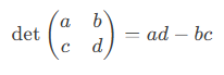
1. • 3×3 Matrix (Sarrus’ Rule):

1. • n×n Matrix: Computed via LU decomposition in Excel.
2. Critical Interpretation:
   • det = 0 → Matrix is singular (no inverse, linearly dependent rows/columns).
   • det ≠ 0 → Matrix is invertible.

Examples

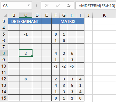
1. Real-World Use:
   • Check invertibility before using MINVERSE().
   • Solve linear systems (Cramer’s Rule).

Why This Matters

• Engineering: Stability analysis of systems.
• Economics: Input-output models.
• Computer Graphics: Transformation matrices.

Error Handling

Error	Cause	Solution
#VALUE!	Non-square/non-numeric input	Ensure square numeric matrix

 

Its returns the common logarithm (base 10) of a positive real number.

Syntax

LOG10(number)

Argument

Parameter	Requirement	Valid Input
number	Required	Positive real number (> 0)

Key Properties

1. Mathematical Definition:

1. • Special Values:
     • LOG10(1) = 0
     • LOG10(10) = 1
     • LOG10(100) = 2
2. Error Handling:
   • #NUM! → number ≤ 0
   • #VALUE! → Non-numeric inputs
3. Inverse Relationship:
   • =10^LOG10(x) returns x
   • =LOG10(10^x) returns x

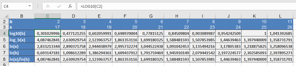
Examples

1. Basic Calculations:

=LOG10(2)  → Returns 0.301029996 

=LOG10(6)  → Returns 0.77815125 

=LOG10(9)  → Returns 0.954242509 

=LOG10(10) → Returns 1 

1. Scientific Applications:
   • Decibels (Sound): =10*LOG10(Power_ratio)
   • pH Scale: =-LOG10(H+_concentration)
   • Richter Scale (Earthquakes): Logarithmic magnitude

Comparison with Other Logs

Function	Base	Example
LOG10()	10	=LOG10(1000) = 3
LN()	*e*	=LN(10) ≈ 2.302585
LOG()	Custom	=LOG(8, 2) = 3

 

Its returns the logarithm of a number to a specified base. If the base is omitted, it defaults to 10 (common logarithm).

Syntax

LOG(number; [base])

Arguments

Parameter	Requirement	Valid Input
number	Required	Positive real number (> 0)
[base]	Optional	Positive real number ≠ 1 (default = 10)

Key Concepts

1. Mathematical Definition:

1. • Inverse of Exponentiation: LOG(number, base) reverses base^y = number.
   • Special Cases:
     • LOG(10) = LOG10(10) = 1 (base 10)
     • LOG(8, 2) = 3 (since 23=823=8)
2. Error Handling:
   • #NUM! → number ≤ 0 or base ≤ 0 / base = 1
   • #VALUE! → Non-numeric inputs

Examples

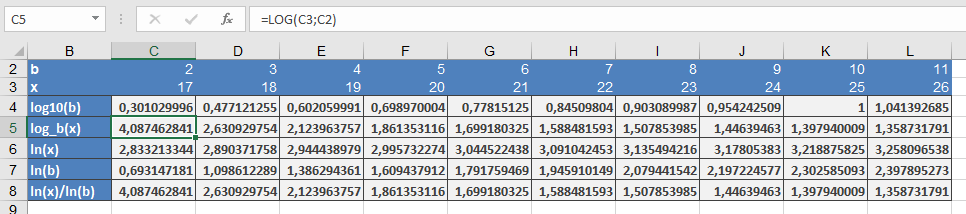
Comparison with Other Log Functions

Function	Base	Example
LOG()	Custom	=LOG(27, 3) → 3
LOG10()	10	=LOG10(1000) → 3
LN()	*e*	=LN(20) ≈ 3.0

Why This Matters

• Simplifies multiplicative problems into additive ones (e.g., compounding interest).
• Essential in data science (log-scaling) and engineering (signal processing).
• Base 2 is critical in computer science (binary trees, Big-O notation).

Common Errors & Fixes

Error	Cause	Solution
#NUM!	number ≤ 0 or invalid base	Ensure inputs are positive and base ≠ 1
#VALUE!	Text input	Use =IFERROR(LOG(A1,B1), « Check Input »)

 

Its returns the natural logarithm (base *e*) of a positive real number, where *e* ≈ 2.71828182845904 (Euler’s number).

Syntax

LN(number)

Argument

Parameter	Requirement	Valid Input
number	Required	Positive real number (> 0)

Key Concepts

1. Mathematical Definition:

1. • Inverse of EXP(): LN(EXP(x)) = x and EXP(LN(x)) = x
   • Special Values:
     • LN(1) = 0
     • LN(e) = 1
2. Error Handling:
   • Returns #NUM! if number ≤ 0
   • Returns #VALUE! for non-numeric inputs
3. Comparison with Other Logs:

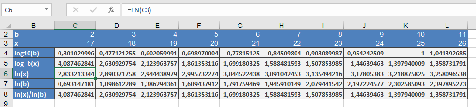
Function	Base	Example
LN()	*e*	=LN(10) ≈ 2.302585
LOG10()	10	=LOG10(100) = 2
LOG()	Custom	=LOG(8,2) = 3

Examples

Why This Matters

The natural logarithm is fundamental in:

• Calculus: Derivatives/integrals of exponential functions
• Physics: Describes natural growth/decay (e.g., Newton’s Law of Cooling)
• Economics: Logarithmic returns in finance

Common Errors & Fixes

Error	Cause	Solution
#NUM!	number ≤ 0	Ensure input is positive
#VALUE!	Text input	Verify numeric values

 

This function rounds a number down to the nearest integer (toward negative infinity).

Syntax
INT(number)

Argument

• number (required) – Any real number to be rounded

Key Behavior:

• Positive numbers: Removes decimal portion (truncates)
  • =INT(3.7) → 3
• Negative numbers: Rounds to next lower integer
  • =INT(-2.3) → -3
• Whole numbers: Returns unchanged
  • =INT(5) → 5

Comparison with Similar Functions:

Function	4.3	-4.3	Behavior
INT()	4	-5	Toward -∞
TRUNC()	4	-4	Toward zero
ROUNDDOWN()	4	-4	Toward zero
FLOOR()	4	-5	Toward -∞ (with significance=1)

Examples:

1. Tax Calculation (Conservative rounding):

=INT(12.78) → 12

1. Special Cases:

Formula	Result	Notes
=INT(4.3)	4	Truncates decimals
=INT(-2.51)	-3	Rounds down
=INT(78.8)	78
=INT(0.999)	0

Applications:

• Financial reporting (conservative estimates)
• Age calculations (whole years)
• Inventory management (whole units)
• Time tracking (complete hours)

Error Handling:

• Returns #VALUE! for non-numeric inputs
• Handles very large/small numbers within Excel’s limits

Technical Notes:

• Differs from TRUNC() for negative numbers
• Equivalent to FLOOR(number,1) for positive numbers
• For rounding to other multiples, consider FLOOR() or CEILING()

This function returns the largest positive integer that divides all specified numbers without a remainder.

Syntax
GCD(number1; [number2]; …)

Arguments

• number1 (required) – First integer value
• number2,… (optional) – Additional integers (up to 255 total values in modern Excel)

Key Features:

• Truncates decimal values to integers
• Requires all arguments ≥ 0 (#NUM! error if negative)
• Returns 0 if all arguments are 0
• At least one non-zero value required for meaningful result

Calculation Methods:

1. Prime Factorization

1. Euclidean Algorithm (More efficient):

Applications:

• Optimizing material cuts (construction/design)
• Fraction simplification (mathematics)
• Cryptography algorithms
• Scheduling recurring events
• Musical rhythm patterns

Error Handling:

=IFERROR(GCD(A1,B1), »Invalid input »)

Related Functions:

• LCM(): Least Common Multiple
• MOD(): Modulus/Remainder
• QUOTIENT(): Integer division