Votre panier est actuellement vide !
Étiquette : function
How to use the PERCENTRANK.EXC() function in Excel
This function returns the rank of a value (alpha) in a dataset as a percentage, ranging from 0 to 1 (exclusive).
Syntax:
PERCENTRANK.EXC(array; x; [significance])Arguments:
- array(required): The array or range of numeric data that defines the relative positions.
- x(required): The value for which you want to determine the rank.
- significance(optional): A value specifying the number of decimal places for the returned percentage. If omitted, EXC() defaults to three decimal places (0.xxx).
Background:
PERCENTRANK.EXC() and PERCENTRANK.INC() are the inverse functions of PERCENTILE.EXC() and PERCENTILE.INC(). These functions calculate the relative position of a value *x* within a dataset.
For additional details on quantiles, refer to the PERCENTILE() documentation.Example:
For more details on how to use this function, see the figure below.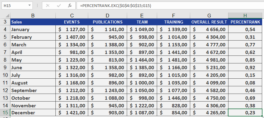
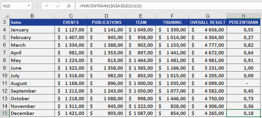
How to use the PERCENTRANK() function in Excel
This function returns the rank of a value (alpha) as a percentage. It can be used to evaluate the relative position of a value within a dataset. For example, you can use PERCENTRANK() to assess the standing of an aptitude test score compared to all other test scores.
Syntax:
PERCENTRANK(array; x; [significance])Arguments:
- array(required): The array or range of numeric data that defines the relative positions.
- x(required): The value for which you want to determine the rank.
- significance(optional): A value specifying the number of decimal places for the returned percentage. If omitted, PERCENTRANK() defaults to three decimal places (0.xxx).
Background:
PERCENTRANK() is the inverse of PERCENTILE(). It calculates the relative position of a value *x* within a dataset. For more details on quantiles, refer to the PERCENTILE() documentation.Example:
As the manager of the controlling department, you want to analyze the annual sales of all business units. Your goal is to determine the percentile rank of a given month’s sales compared to all monthly sales on a scale from 1 to 100, helping you assess sales variance.Using PERCENTRANK(), you find that January’s sales of $4,656.00 have a quantile rank of 0.55. This means:
- The sales value ranks at 55on a scale of 1 to 100.
- 55%of all monthly sales are less than or equal to $4,656.00, while 45% are greater than or equal to this value (see Figure below).
How to use the PERCENTILE() function in Excel
Returns the alpha quantile (a threshold value) of a dataset, where alpha is a decimal between 0 and 1. This helps identify cutoff points (e.g., « Top 20% of sales »).
Syntax:
PERCENTILE(array; alpha)
Arguments:
- array (required) – The dataset (numeric range) to analyze.
- alpha (required) – The percentile (e.g., 0.8 for 80th percentile).
Background:
- Quantiles split data into ordered segments:
- Median = 0.5 quantile (50th percentile).
- Quartiles = 0.25, 0.5, 0.75 quantiles.
- Deciles = 0.1, 0.2, …, 0.9 quantiles.
- Calculation Rules:
- If n * alpha is not an integer, round up to the next data point.
- If n * alpha is an integer, interpolate between adjacent values.
(Example: For 16 data points, the 0.25 quantile falls between the 4th and 5th values.)
Example:
A software company analyzes annual sales across business units to identify top performers:
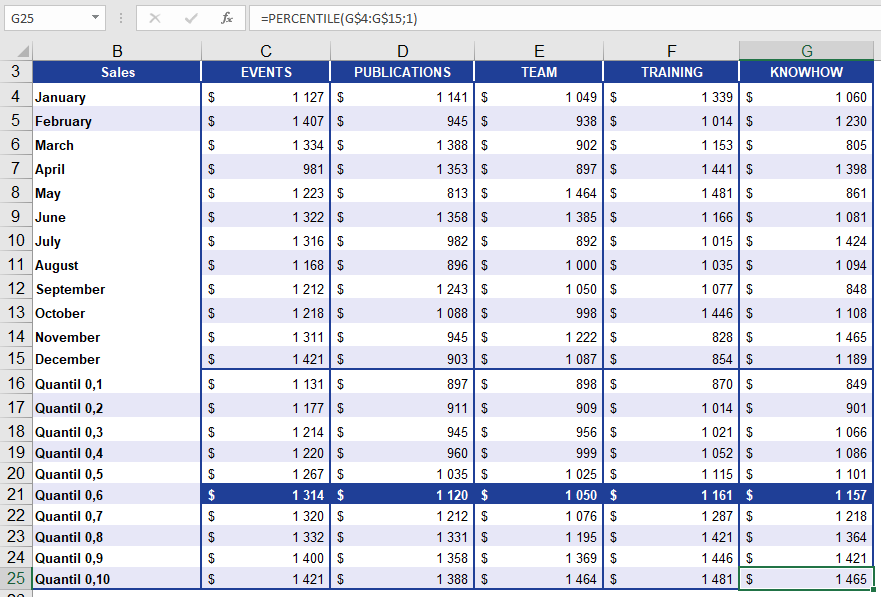
- 60% of sales values are below the returned threshold.
- 40% of sales values are at or above it.
Key Notes:
- Practical Use: Flag high-performing segments (e.g., « Invite customers above the 80th percentile to an event »).
- Limitation: Requires sorted data for manual validation.
How to use the PEARSON() function in Excel
Returns the Pearson correlation coefficient (*r*), a dimensionless value between –1.0 and 1.0 that quantifies the linear relationship between two datasets.
Syntax:
PEARSON(array1; array2)
Arguments:
- array1 (required) – Independent variable (*x*) values.
- array2 (required) – Dependent variable (*y*) values.
Background:
- Interpretation of *r*:
- +1: Perfect positive linear correlation.
- –1: Perfect negative linear correlation.
- 0: No linear correlation.
- Limitations:
- Only measures linear relationships (ignores nonlinear patterns).
- Does not imply causation.
- Formula:
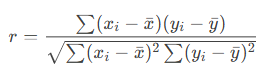
Where xˉ and yˉ are the means of array1 and array2.
Example:
A software company analyzes the relationship between website visits (x) and online orders (y).
- Scatter Plot (Figure below): Visual linear trend suggests correlation.
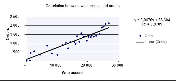
- Calculation:
=PEARSON(B2:B100, C2:C100) // Returns r = 0.933
Result (Figure below):
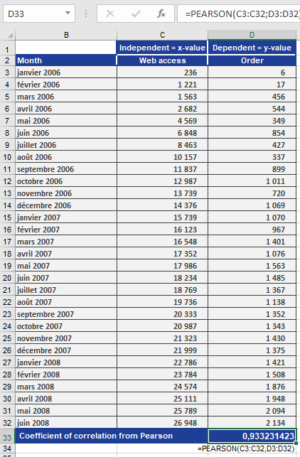
-
- r=0.933r=0.933 → Strong positive correlation.
- Interpretation: Increased website visits closely align with increased orders.
Key Notes:
- High *r* ≠ Causation: Confounding factors (e.g., marketing campaigns) may influence results.
- Always visualize data (e.g., scatter plots) to validate linearity.
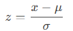
How to use the NORM.S.INV() function in Excel
This function returns the z-value (quantile) of the standard normal distribution (mean = 0, standard deviation = 1) for a given cumulative probability.
Syntax:
NORM.S.INV(probability)
Arguments:
- probability (required) – A cumulative probability (0 < p < 1) associated with the standard normal distribution.
Background:
- The NORM.S.INV() function is the inverse of NORM.S.DIST().
- It calculates the z-value (standardized score) corresponding to a given cumulative probability (area under the curve to the left of *z*).
- The standard normal distribution has:
- Mean (μ) = 0
- Standard deviation (σ) = 1
Example:
Using the light bulb lifespan data from previous examples (STANDARDIZE() and NORM.S.DIST()):
- You have already calculated probabilities for performance values (see Figure below).
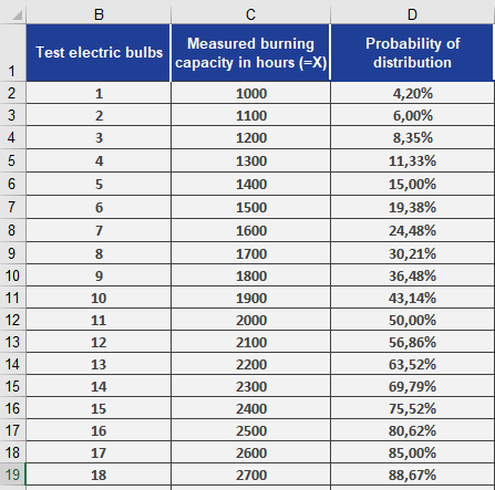
- To find the z-values for these probabilities:
=NORM.S.INV(D2) // Returns z-value for the probability in cell D2
Results (see Figure below):
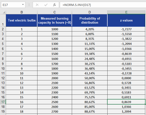
- The function converts probabilities (e.g., 0.042) back to their standard normal distributed z-values (e.g., –1.728).
- Interpretation: A probability of 4.2% corresponds to z = –1.728, meaning 4.2% of bulbs fall below this standardized lifespan.
Key Notes:
- Inverse Function: Maps probabilities back to z-scores, unlike NORM.S.DIST() (which maps z-scores to probabilities).
- Standard Normal Only: Assumes μ = 0 and σ = 1 (use NORM.INV() for non-standard distributions).
How to use the NORM.S.DIST() function in Excel
This function returns the probability (either cumulative or density) for a given z-value in the standard normal distribution (mean = 0, standard deviation = 1). It eliminates the need for traditional statistical tables.
Syntax:
NORM.S.DIST(z ; cumulative)
Arguments:
- z (required) – The quantile (standardized value) for which the probability is calculated.
- cumulative (required) – A logical value determining the output:
- TRUE: Returns the cumulative distribution function (CDF).
- FALSE: Returns the probability density function (PDF).
Background:
The standard normal distribution has:
- Mean (μ) = 0
- Standard deviation (σ) = 1
Its density function is given by:
- CDF (cumulative = TRUE): Returns P(Z≤z)(e.g., the area under the curve to the left of *z*).
- PDF (cumulative = FALSE): Returns the height of the curve at *z*.
Example:
Using the light bulb lifespan data from the STANDARDIZE() example:
- Measurements are standardized to z-values (e.g., –1.728 in cell D2).
- To find the probability for each z-value:
=NORM.S.DIST(D2, TRUE) // Returns cumulative probability
Results (see Figure below):
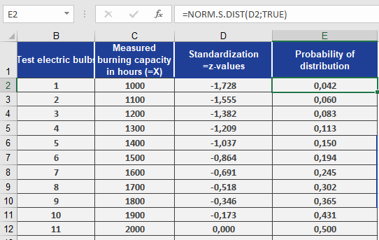
- For z = –1.728, the probability is 4.2% (cell E2).
Interpretation: Only 4.2% of bulbs have a lifespan ≤ this z-value.
How to use the NORMINV() function in Excel
This function returns the quantile (inverse of the cumulative distribution) of a normal distribution for a given probability, mean, and standard deviation.
Syntax:
NORMINV(probability; mean; standard_dev)
Arguments:
- probability (required) – A probability value (0 ≤ *p* ≤ 1) associated with the normal distribution.
- mean (required) – The arithmetic mean (µ) of the distribution.
- standard_dev (required) – The standard deviation (σ) of the distribution.
Background:
A standard normal distribution has:
- Mean (µ) = 0
- Standard deviation (σ) = 1
Any normal distribution can be converted to a standard normal distribution using:
Conversely, a value () in a normal distribution can be derived from a z-score using:
x=μ+z⋅σ
For the standard normal distribution (see Figure below):
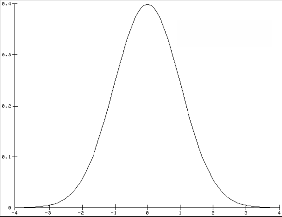
- 68% of values fall within ±1σ of the mean.
- 95.5% of values fall within ±2σ of the mean.
- 99.7% of values fall within ±3σ of the mean.
These same percentages apply to all normal distributions, regardless of µ and σ.
Example:
You are a light bulb manufacturer analyzing lifespan data:
- Mean (µ) = 2,000 hours
- Standard deviation (σ) = 579 hours
You want to find the lifespans for the top 85% and bottom 15% of bulbs.
Using NORMINV():
- 85th percentile: =NORMINV(0.85, 2000, 579) → ~2,600 hours
- 15th percentile: =NORMINV(0.15, 2000, 579) → ~1,400 hours
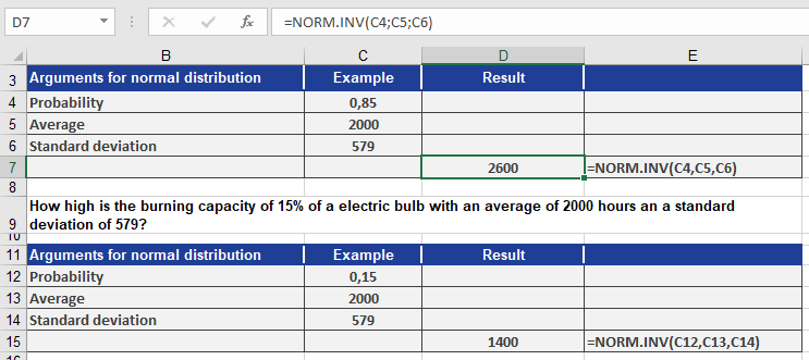
Interpretation (see Figure above):
- 85% of bulbs last up to 2,600 hours.
- 15% of bulbs last up to 1,400 hours.
How to use the NORM.DIST() function in Excel
This function returns the normal distribution for a specified average value and standard deviation. It has broad applications in statistics, including hypothesis testing.
Syntax. NORM.DIST(x, mean, standard_dev, cumulative)
Arguments
- x (required): The distribution value (quantile) for which you want to calculate the probability.
- mean (required): The arithmetic mean of the distribution.
- standard_dev (required): The standard deviation of the distribution.
- cumulative (required): A logical value indicating the type of distribution:
- If TRUE, the function returns the cumulative distribution function (CDF).
- If FALSE, the function returns the probability density function (PDF).
Background.
Excel provides numerous statistical functions to calculate distributions and test hypotheses. One such function is NORM.DIST(). In general, distribution functions help answer probability-related questions.For example, a coin toss has two outcomes: heads or tails.
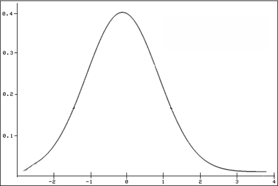
The NORM.DIST() function specifically returns the normal distribution of a given value. The normal distribution is the most important continuous probability distribution, indicating the probability of a random variable x. This distribution is also referred to as the Gaussian function, Gaussian bell, or bell curve, and is shown in Figure beow.
Mathematical Formula (for cumulative = FALSE):
The probability density function (PDF) of the normal distribution is:
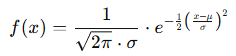
Where:
- x = value in the distribution (quantile)
- μ = mean (average)
- σ = standard deviation
- e = Euler’s number (approx. 2.71828)
If cumulative = TRUE, the formula computes the integral of the above expression from negative infinity up to xxx, yielding the cumulative probability.
Additional Notes on the Normal Distribution:
- It is bell-shaped.
- It is unimodal (has one peak).
- It is symmetrical around the mean.
- It asymptotically approaches the x-axis.
- The maximum occurs at the mean.
- 50% of values lie on either side of the mean.
- Mean, median, and mode are equal.
- Inflection points are located at μ±σ\mu \pm \sigmaμ±σ.
Excel provides both:
- A function ending in DIST to calculate the probability of a value.
- A function ending in INV to calculate the value for a given probability.
Example.
You’re a light bulb manufacturer analyzing bulb lifespans. You’ve determined:- Mean (μ) = 2,000 hours
- Standard Deviation (σ) = 579 hours
You use NORM.DIST() to evaluate the probability that a bulb lasts:
- Up to 2,600 hours
- Only 1,400 hours
Use:
- cumulative = TRUE → for cumulative probability
- cumulative = FALSE → for exact probability (density)
So for:
- x=2,600x = 2,600x=2,600, NORM.DIST(2600, 2000, 579, TRUE)
- x=1,400x = 1,400x=1,400, NORM.DIST(1400, 2000, 579, TRUE)
- Exact: use the same x values, but set cumulative = FALSE.
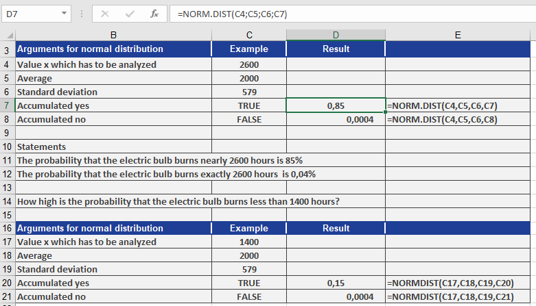
Conclusions from Figure above:
- The probability a light bulb works up to 2,600 hours: 85%
- The probability it works exactly 2,600 hours: 0.04%
- The probability it works only 1,400 hours: 15%
- The probability it works exactly 1,400 hours: 0.04%
With this method, you can:
- Perform hypothesis tests
- Calculate probabilities
- Determine value ranges for various confidence intervals
How to use the NEGBINOM.DIST() function in Excel
This function returns the probability of a negatively binomial-distributed random variable. NEGBINOM.DIST() calculates the probability that there will be number_f failures before the number_s-th success occurs, given a constant probability of success probability_s.
Syntax
NEGBINOM.DIST(number_f; number_s; probability_s)
Arguments
- number_f (required): The number of failures
- number_s (required): The number of successes
- probability_s (required): The probability of a success
Background. This function is similar to the binomial distribution, except that the number of successes is fixed and the number of trials is variable. This is known as a negative binomial distribution. As with the binomial distribution, trials are assumed to be independent.
In a random experiment involving independent repetitions with only two possible outcomes (success or failure), the negative binomial distribution (also known as the Pascal distribution) returns the probability of a fixed number of failures before the x-th success. The formula for the negative binomial distribution is:
where:
- x = number_f
- r = number_s
- p = probability_s
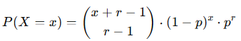
Example. You are on vacation in a foreign city and ask a passerby for directions. Each response can only be « yes » or « no », meaning there is a 50% probability that the answer is « yes ». Therefore, p = 0.5.
After asking several people and receiving no helpful answers, you decide to buy a map. Now, you’re interested in knowing the probability of receiving several “No, I’m sorry” responses before encountering five people who can help. You use the NEGBINOM.DIST() function to calculate this probability, as shown in Figure below.
From the result, you can conclude:
With number_f = 6, the probability of asking six people who don’t know the way before you find five people who do is 10.25%.How to use the MODE.SNGL() function in Excel
Returns the most frequently occurring value in a dataset. If multiple values have the same highest frequency, it returns the first one encountered.
Syntax
MODE.SNGL(number1; [number2]; …)
Arguments
- number1 (required): First number, cell reference, or range
- number2,… (optional): Additional values/ranges
Key Features
- Data Handling:
- Only considers numeric values
- Ignores:
- Empty cells
- Text entries
- Logical values
- Returns #N/A if no duplicates exist
- Comparison with Other Measures:
Measure Returns When to Use MODE.SNGL Most common value Identifying frequent outcomes MEDIAN Middle value Skewed distributions AVERAGE Arithmetic mean Normally distributed data Example. You are the sales manager of the software company and want to evaluate the number of visits your sales representatives made in different regions numbered 1 through 5: Texas, Virginia, California, Oregon, and Washington. You have already created a table (see figure below).
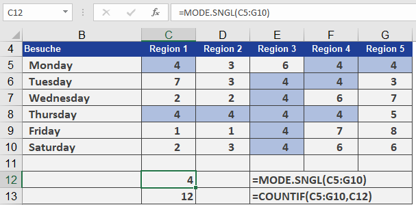
You want to know how many visits were usually necessary before a contract was signed. For this you use the MODE.SNGL() function.
Most of the time, it took four visits to get to the point where the customer signed the contract. If you nest the COUNTIF() and MODE.SNGL() functions, you can also count the number of modes in the range.