Votre panier est actuellement vide !
Étiquette : statistical
How to use the INTERCEPT() function in Excel
Calculates the y-intercept of the linear regression line fitted to a dataset. This is the point where the regression line crosses the y-axis (i.e., the predicted value of y when x = 0).
Syntax:
INTERCEPT(known_y’s; known_x’s)Arguments
Argument Required? Description known_y’s Yes Dependent variable (response data). Must be a single row/column. known_x’s Yes Independent variable (predictor data). Must match dimensions of known_y’s. Error Handling:
- Returns #N/A if:
- known_y’s and known_x’s have unequal lengths.
- Either argument is empty.
Background
Regression Analysis Context:
- Models the linear relationship between dependent (y) and independent (x) variables.
- The regression line minimizes the sum of squared deviations (least squares method).
Equation of the Line:
y=mx+b
Where:
- b= y-intercept (calculated by INTERCEPT()).
- m = slope (calculated by SLOPE()).
Intercept Formula:
b=yˉ−mxˉ
- yˉ: Mean of known_y’s.
- xˉ: Mean of known_x’s.
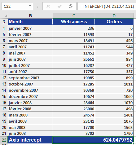
Example: Website Traffic Analysis
Scenario:
A company analyzes if orders (y) depend on website visits (x) (Jan 2007–Jun 2008).Step 1: Calculate Intercept
=INTERCEPT(orders_range ; visits_range)
Result: 524.05 (see Figure below).
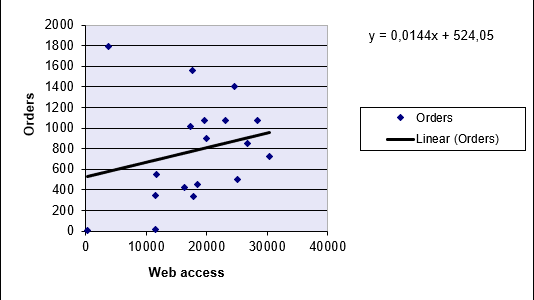
Step 2: Interpret Results
- The intercept (b = 524.05) implies:
- If there are zero visits, the model predicts 524 orders (theoretical baseline).
- Combined with the slope (m), it defines the regression line equation.
Visualization:
- A scatter plot with a trendline shows the intercept at y = 524.05 (Figure below).
Key Notes
- Usage with SLOPE():
- Use both functions to fully define the regression line:
y = SLOPE(y’s, x’s) * x + INTERCEPT(y’s, x’s)
- Assumptions:
- Linear relationship between x and y.
- Homoscedasticity (constant variance of residuals).
- Practical Applications:
- Forecasting sales based on advertising spend.
- Predicting exam scores from study hours.
- Returns #N/A if:
How to use the HYPGEOM.DIST() function in Excel
This function returns probabilities for a hypergeometrically distributed random variable. It calculates the probability of obtaining a specific number of successes in a sample drawn from a finite population without replacement.
Syntax:
HYPGEOM.DIST(sample_s; number_sample; population_s; number_population; cumulative)Required Information:
- Number of successes in the sample
- Size of the sample
- Number of possible successes in the population
- Size of the population
- Logical value determining the function type
Arguments
- sample_s (required): The number of successes in the sample.
- number_sample (required): The size of the sample.
- population_s (required): The number of successes in the population.
- number_population (required): The total size of the population.
- cumulative (required): A logical value that determines the function form:
- FALSE: Returns the probability mass function (exact probability).
- TRUE: Returns the cumulative distribution function.
Background
The hypergeometric distribution answers: « What is the probability of finding x successes in a sample drawn from a finite population? »
Key Characteristics:
- Used when sampling without replacement from a finite population.
- Each observation is either a success or failure.
- Subsets are chosen with equal likelihood.
Equation:
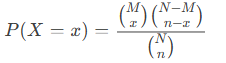
Where:
- x=sample_s
- n=number_sample
- M=population_s
- N=number_population
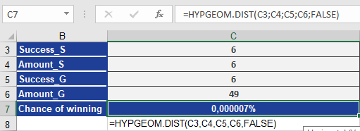
Example: Lottery Probability
Scenario: Calculate the probability of winning a lottery with 6 numbers drawn from 49.
Arguments:
- sample_s = 6 (winning numbers in ticket)
- number_sample = 6 (numbers drawn)
- population_s = 6 (total winning numbers)
- number_population = 49 (total balls)
- cumulative = FALSE (exact probability)
Calculations:
- Probability of 6/6 (Jackpot):
=HYPGEOM.DIST(6, 6, 6, 49, FALSE) → 0.00000715% (Figure below).
- Probabilities for Smaller Wins:
- 5/6: =HYPGEOM.DIST(5, 6, 6, 49, FALSE) → 0.0018%
- 4/6: =HYPGEOM.DIST(4, 6, 6, 49, FALSE) → 0.10%
- 3/6: =HYPGEOM.DIST(3, 6, 6, 49, FALSE) → 1.77% (Figure below).
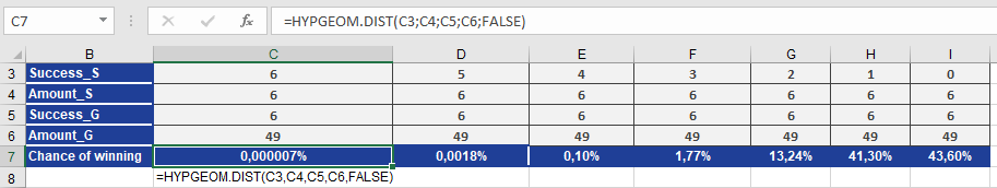
Conclusion:
The hypergeometric distribution precisely models scenarios with finite populations and without replacement, such as lotteries or quality control testing.How to use the HARMEAN() function in Excel
Returns the harmonic mean of a dataset, which is the reciprocal of the arithmetic average of reciprocals.
Syntax:
HARMEAN(number1; [number2]; …)Arguments
- number1 (required) – First value or range for calculation.
- number2, … (optional) – Additional values or ranges.
- Can use a single array (e.g., A1:A5) instead of comma-separated values.
Background
The harmonic mean is used for:
- Averaging rates or ratios (e.g., speed = distance/time).
- Cases where values are defined by reciprocal relationships.
Equation:
Harmonic Mean=n1x1+1×2+⋯+1xnHarmonic Mean=x11+x21+⋯+xn1n
where n = number of values, x = data points.
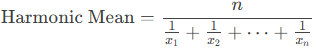
Example. To explain how the harmonic mean is calculated, use the previously mentioned example of speed and time. A bicyclist travels 300
miles through the Alps. The distance is divided into five legs, for which he measures the speed of each.
Now the bicyclist wants to calculate the average speed from the speeds reached in each leg. The result should show the consistent speed at which he could have traveled the same distance in the same time (see Figure below).
To get a better overview, he also calculated the arithmetic average and the geometric mean.
To find out what calculation returns the best result, he transforms the results of the arithmetic, geometric, and harmonic means in meters/seconds and then calculates the time it would take to travel the 300 miles at the average speed (see figure below).

This calculation also confirms that the geometric mean is smaller than the harmonic mean, and the arithmetic mean is smaller than the geometric mean.
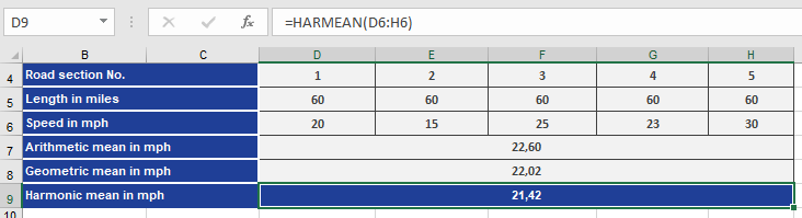
Next, you prove that the harmonic mean returns the best result. First you have to calculate speed v in m/s for the actual miles travelled at speed v for each leg in an hour. At a steady speed, the cyclist could have traveled 20 miles per hour in the first leg. If you divide 20 miles by 3,600 seconds, you get the speed v (see figure below).
Where V=S/t
Then you use the result for the speed in m/s in the same formula for t (time) to calculate the time for each leg in seconds. Given the fomular
t=S/V
the figure below shows the result.
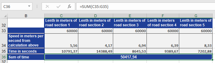
The sum of the times in seconds for the legs shows that the value is approximately the same as the harmonic mean. The difference of three seconds is based on the rounded values.
The comparison of the actual result of 50,417.94 seconds with the calculated results of the different means shows that the harmonic mean returns the best result.
Conclusion: The harmonic mean gives the most accurate average for rates.
How to use the GROWTH() function in Excel
The GROWTH function calculates predicted values based on an exponential trend. It returns y-values corresponding to a specified set of new x-values using existing x and y data. It can also fit an exponential curve to known data points.
Syntax:
GROWTH(known_y’s; known_x’s; new_x’s; const)Arguments
- known_y’s (required) – The dependent y-values from the exponential relationship y = b * m^x.
- If known_y’s is a single column, each column in known_x’s is treated as an independent variable.
- If known_y’s is a single row, each row in known_x’s is treated as an independent variable.
- known_x’s (optional) – The independent x-values from the relationship y = b * m^x.
- Supports single or multiple variable sets. If only one variable is used, known_y’s and known_x’s can be any shape but must have matching dimensions. For multiple variables, known_y’s must be a vector (single row or column).
- If omitted, defaults to {1, 2, 3, …} with the same length as known_y’s.
- Requirements:
- known_y’s and known_x’s must have the same number of rows/columns. A mismatch returns #REF!.
- Any zero or negative y-value returns #NUM!.
- new_x’s (optional) – New x-values for which to predict y-values.
- Must match known_x’s in structure:
- If known_y’s is a column, new_x’s must have the same columns.
- If known_y’s is a row, new_x’s must have the same rows.
- If omitted, defaults to known_x’s.
- If both known_x’s and new_x’s are omitted, they default to {1, 2, 3, …} (same length as known_y’s).
- Must match known_x’s in structure:
- const (optional) – Logical value controlling the constant b in y = b * m^x:
- TRUE (or omitted): Calculates b normally.
- FALSE: Forces b = 1, adjusting m to fit y = m^x.
Background
While TREND() models linear trends, GROWTH() fits exponential trends, useful when data grows by a fixed factor or percentage. It projects future values by fitting an exponential curve to historical data.
Example
A marketing manager analyzes website visits and online orders (Figure below), which grew exponentially from January 2007–June 2008. To forecast July 2008–March 2009:
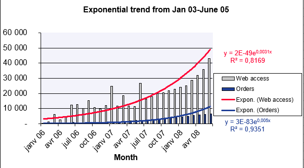
Website Visits Forecast
- known_y’s: Visits (Jan–Jun 2008).
- known_x’s: Months (Jan 2006–Jun 2008).
- new_x’s: Months (Jul 2008–Mar 2009).
- const: TRUE (calculate b normally).
Result: Predicted values shown in Figure below.
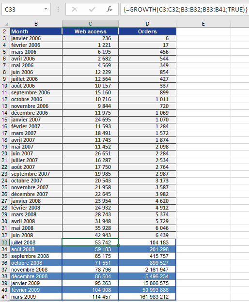
Online Orders Forecast
Using the same method, orders are projected (Figure below).

Conclusion
GROWTH() provides accurate exponential trend forecasts, assuming historical growth patterns continue.
- known_y’s (required) – The dependent y-values from the exponential relationship y = b * m^x.
How to use the GEOMEAN() function in Excel
This function returns the geometric mean of a set of positive numbers. The geometric mean is particularly useful for calculating average growth rates (e.g., compound interest, variable returns, or percentage-based trends).
The geometric mean is computed as the n-th root of the product of all values, where n is the number of values:

Syntax:
GEOMEAN(number1; [number2]; …)
Arguments:
- number1 (required) – The first number or range for calculation.
- number2, … (optional) – Additional numbers or ranges (up to 255 in modern Excel).
- Note: Arguments can be supplied as individual values, arrays, or cell references.
Background:
The geometric mean is ideal for analyzing percentage-based changes (e.g., growth rates, inflation, or multiplicative processes), where the arithmetic mean would produce misleading results.
Example:
Scenario:
As a controlling manager at a software company, you want to determine the average monthly sales growth rate over a period.Problem:
- Using the arithmetic mean would overestimate growth (e.g., showing 113% average growth).
- The geometric mean correctly reflects the compounded trend, revealing an average 97% growth factor (i.e., a 3% decline).
Steps:
- Calculate monthly growth factors (current month / previous month).
- Apply GEOMEAN() to these factors to derive the true average growth rate.
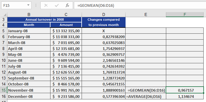
Result:
The geometric mean (97%) indicates a net decline, while the arithmetic mean (113%) falsely suggests growth.Key Insight:
- Geometric mean = Accurate for multiplicative processes (e.g., finance, biology).
- Arithmetic mean = Misleading for volatile or percentage-based data.
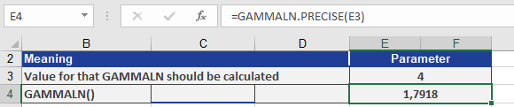
How to use the GAMMALN.PRECISE() function in Excel
This function returns the natural logarithm of the gamma function, Γ(x), calculated with 15-digit precision.
Syntax:
=GAMMALN.PRECISE(x)
Arguments:
- x (required) – The value for which you want to calculate GAMMALN.PRECISE().
Background:
For background details, refer to the documentation for the GAMMALN() function.
Example:
For usage examples demonstrating the GAMMALN.PRECISE functions below;
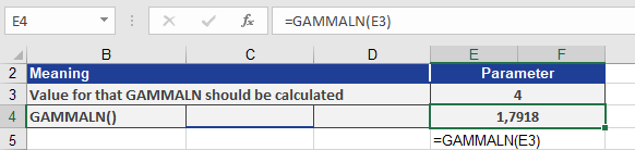
How to use the GAMMALN() function in Excel
This function returns the natural logarithm of the gamma function, Γ(*x*).
Syntax:
GAMMALN(x)
Arguments:
- x (required) – The value for which you want to calculate GAMMALN().
Background:
The GAMMALN() function returns the natural logarithm (base *e*) of the gamma function.
A logarithm of a number is the exponent to which a fixed base must be raised to produce that number. Common logarithms include:
- Natural logarithm (ln): Base *e* (Euler’s number ≈ 2.71828)
- Base-10 logarithm (log₁₀)
- Base-2 logarithm (log₂)
The logarithm (to base *b*) of a number *y* is the exponent by which *b* must be raised to obtain *y*. Thus, the logarithmic function is the inverse of the exponential function.
Calculation:
GAMMALN(x) is computed as:
ln(Γ(x))ln(Γ(x))

where Γ(x) is the gamma function.
Example:
To calculate GAMMALN(4), refer to Figure below, which illustrates the computation.
The GAMMALN() function returns the natural logarithm 1.7918 for the gamma function evaluated at *x* = 4.
How to use the GAMMA.DIST() function in Excel
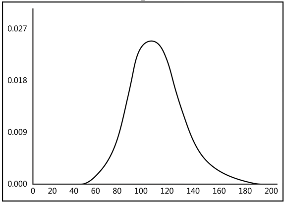
This function returns the probabilities of a gamma-distributed random variable. It is used to analyze variables with a skewed distribution, commonly applied in queuing theory and other statistical analyses.
Syntax
GAMMA.DIST(x; alpha; beta; cumulative)
Arguments
- x (required) – The value (quantile) for which the probability is calculated.
- alpha (required) – A shape parameter of the distribution.
- beta (required) – A scale parameter of the distribution. If beta = 1, the function returns the standard gamma distribution.
- cumulative (required) – A logical value determining the function type:
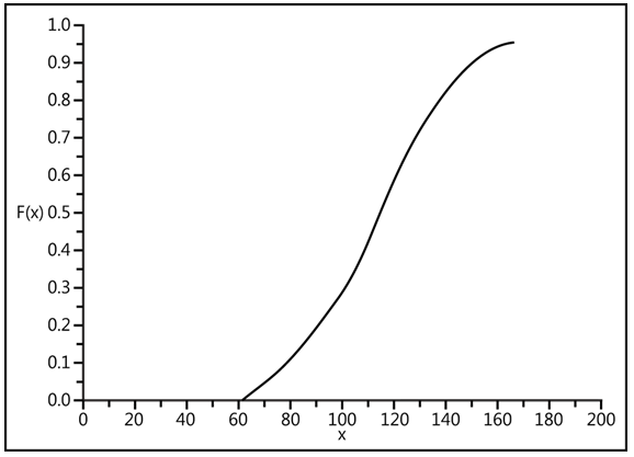
- If TRUE, GAMMA.DIST() returns the cumulative distribution function (probability that a random event occurs between 0 and x).
- If FALSE, it returns the probability density function.
Background
The gamma distribution is a continuous probability distribution for positive real numbers (see Figure below). Its probability density function is defined for x > 0, with f(x) = 0 for other values.
Key Properties:
- Parameters p (alpha) and q (beta) must be > 0.
- The prefactor bᵖ/Γ(p) ensures correct normalization, where Γ(p) is the gamma function.
- Expected value (mean) = αβ
- Variance = αβ²
Reproductive Property:
- If X and Y are independent gamma-distributed variables with parameters (β, pₓ) and (β, pᵧ), their sum X + Y follows a gamma distribution with parameters (β, pₓ + pᵧ).
Special Cases:
- The chi-square distribution (with k degrees of freedom) is a gamma distribution where p = k/2, β = ½.
- The exponential distribution (with rate λ) is a gamma distribution with p = 1, β = λ.
- The Erlang distribution (with λ and n degrees of freedom) corresponds to p = n, β = λ.
- The quotient X/(X + Y) of two independent gamma-distributed variables follows a beta distribution with parameters pₓ and pᵧ.
Parameterization Note:
- Some literature uses alternative parameterizations (e.g., αβ for mean). To avoid confusion, explicitly state moments (e.g., mean = αβ, variance = αβ²). See Figure below.
Function Details
- GAMMA.DIST() is a two-parameter (alpha, beta) mathematical distribution based on the gamma function.
- It is the inverse of GAMMA.INV().
Example
Calculate GAMMA.DIST() using the following inputs:
- x = 10 (quantile value)
- alpha = 2.70 (shape parameter)
- beta = 2 (scale parameter)
Results (see Figure below):
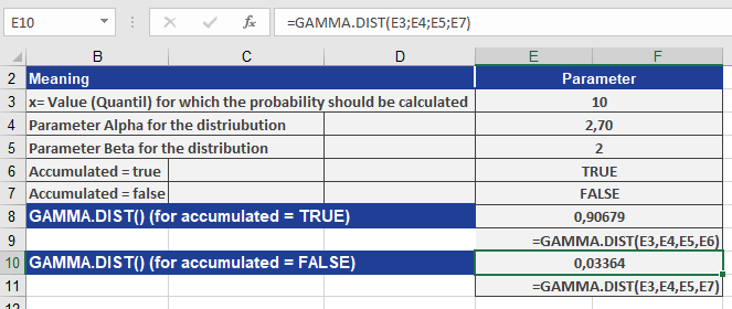
- 0.90679 (cumulative = TRUE)
- 0.03364 (cumulative = FALSE)
Key Takeaways
- The gamma distribution models skewed, positive continuous data.
- Parameters alpha (shape) and beta (scale) define its behavior.
- Cumulative = TRUE returns probabilities (CDF), while FALSE returns density values (PDF).
- Special cases include chi-square, exponential, and Erlang distributions.
This function is essential for advanced statistical modeling, particularly in reliability analysis and stochastic processes.
How to use the GAMMA.INV() function in Excel
This function returns the quantile of the gamma distribution. If
p = GAMMA.DIST(x,…), then GAMMA.INV(p,…) = x.Use this function to examine a variable whose distribution may be skewed.
Syntax:
GAMMA.INV(probability; alpha; beta)Arguments:
- probability(required) – A probability associated with the gamma distribution.
- alpha(required) – A parameter of the distribution.
- beta(required) – A parameter of the distribution. If beta = 1, INV() returns the standard gamma distribution.
Background:
GAMMA.INV() is the inverse function of GAMMA.DIST() and can be used to model a gamma distribution. The alpha and beta arguments correspond to the values for the GAMMA.DIST() function. The probability can be any value from 0 through 100 percent. GAMMA.INV() calculates the position of x on the horizontal axis that matches the cumulative area ratio of the gamma distribution.Example:
Use the values in Figure below to calculate GAMMA.INV(). The figure also shows the calculation of GAMMA.INV().
The GAMMA.INV() function returns the quantile 10 for the gamma distribution based on the parameters shown.
How to use the FREQUENCY() function in Excel
This function returns a frequency distribution as a single-column matrix. For example, use FREQUENCY() to count sales within a specific range. Since FREQUENCY() returns an array of values, it must be entered as an array formula.
Syntax
FREQUENCY(data_array; bins_array)
Arguments
- data_array (required) – An array of or reference to a set of values for which you want to count frequencies. If data_array contains no values, FREQUENCY() returns an array of zeros.
- bins_array (required) – An array of or reference to intervals used to group the values in data_array. If bins_array contains no values, FREQUENCY() returns the number of elements in data_array.
Background
To simplify quantitative data analysis, values are categorized into classes, and their frequencies are calculated. Keep the following in mind:
- Too many classes provide more detail but reduce overall clarity, while too few classes oversimplify the data.
- Classes do not need to be of equal size.
Unlike the COUNTIF() function, FREQUENCY() does not require manual entry in each result cell. Instead, it can be entered once as an array formula, returning results across multiple cells.
Example
We’ll use the example of a software company’s sales data. A sales representative recorded monthly sales over two years in Excel. The manager wants sales categorized as:
- Up to $15,000
- Up to $17,000
- Up to $19,000
- More than $19,000
Thus, four classes are needed.
- The data to be classified is in cells C3:C26 (see Figure below).
- The class intervals are defined in the Class column.
- The frequency of data within each class is calculated based on these intervals.
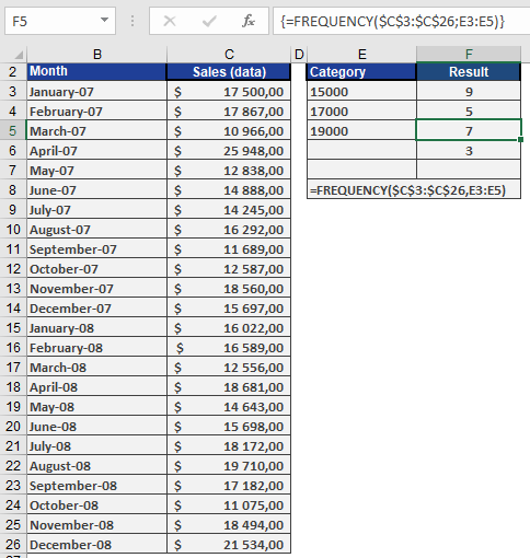
Since FREQUENCY() is an array function, select all four result cells (F3:F6) to display the output as an array.