Étiquette : statistical

The FORECAST() function predicts a future value (y) based on existing linear trends in your data. It uses linear regression to estimate the dependent variable (y) for a given independent variable (x).

Syntax

FORECAST(x; known_y’s; known_x’s)

When to Use

• Predict future sales, inventory needs, or consumer trends.
• Estimate values along a linear trendline.

Arguments

Argument	Required	Description
x	Yes	The data point (independent variable) for which you want to predict a value.
known_y’s	Yes	The dependent data range (values you want to predict, e.g., sales numbers).
known_x’s	Yes	The independent data range (e.g., time periods, ad spend).

Background

How It Works

1. Fits a linear trend (y = mx + b) to your historical data (known_x’s, known_y’s).
2. Predicts y for a new x value along this trendline.

Limitations

• Assumes a linear relationship between x and y.
• For non-linear trends, use GROWTH() (exponential) or TREND() (array-based).

Example: Predicting Website Visits & Online Orders

Scenario

As a marketing director, you want to forecast:

1. Online orders based on predicted visits.

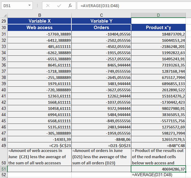
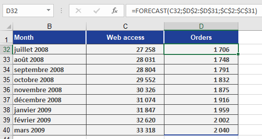
Forecast Online Orders

• x: Predicted visits (C32).
• known_y’s: D2:D31 (Orders from Jan 2005 – Jun 2008).
• known_x’s: C2:C31 (Historical visits).

Formula:

=FORECAST(C32, D2:D31, C2:C31)

Result: Predicts orders for July 2008 (Figure below).

Copying the Formula

Use absolute references (e.g., $C$2:$C$31) to drag the formula across cells D33:D40 for future months.

Key Takeaways

 Best for Linear Trends: Simple, fast predictions when data follows a straight-line pattern.
 Not for Complex Trends: Use TREND() or GROWTH() for non-linear data.
 Workflow:

1. Organize historical x and y data.
2. Apply FORECAST(x, known_y’s, known_x’s).
3. Copy formulas for multiple predictions.

The FISHERINV() function reverts a Fisher-transformed value (y) back to its original correlation coefficient (x). It is the inverse of the FISHER() function, ensuring that:

• If y = FISHER(x), then FISHERINV(y) = x.

Syntax

FISHERINV(y)

Arguments

• y (required): A numeric value representing a Fisher-transformed (z) value that you want to convert back to a correlation coefficient.

Background

Purpose

• Reverses the Fisher Transformation: Converts a normally distributed z-value (from FISHER()) back to a correlation coefficient (r).
• Critical for Averaging Correlations: After averaging Fisher-transformed values, FISHERINV() restores the result to the interpretable -1 to +1 scale.

Mathematical Formula

The inverse Fisher transformation is calculated as:

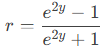
Where:

• y = Fisher-transformed (z) value.
• r = Original correlation coefficient.

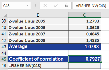
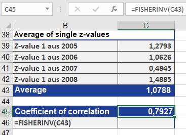
Example

Context

Referencing the FISHER() example:

1. Transformed yearly correlation coefficients (r) into z-values using FISHER().
2. Averaged the z-values.
3. Applied FISHERINV() to revert the averaged z back to a single r (result: 0.7927).

Why This Matters

• Ensures valid interpretation of averaged correlations.
• Preserves the mathematical properties of correlation coefficients.

Key Takeaways

• Use Case: Revert Fisher-transformed data (z) to original correlations (r).
• Pair with FISHER(): Essential for averaging correlations or hypothesis testing.
• Output Range: Returns values between -1 and 1 (standard correlation scale).

Visual Workflow

1. Original r → FISHER(r) → z (normalized).
2. Average z-values.
3. FISHERINV(z_avg) → Final r (interpretable result).

The FISHER() function computes the Fisher transformation of a given value x. This transformation converts a correlation coefficient (which ranges between -1 and +1) into an approximately normally distributed variable, enabling statistical tests on correlation data.

Syntax

FISHER(x)

Arguments

• x (required): A numeric value between -1 and 1 (typically a correlation coefficient r) that you want to transform.

Background

Correlation vs. Regression

• Correlation (r) measures the linear relationship between two variables.
  • Ranges from -1 (perfect negative correlation) to +1 (perfect positive correlation).
  • 0 indicates no linear relationship.
• Regression describes how one variable predicts another, while correlation quantifies their association.

Why Use Fisher Transformation?

1. Non-Interval Scaling:
   • The difference between r=0.2 and r=0.4 is not equivalent to the difference between r=0.4 and r=0.6.
   • Direct averaging of correlation coefficients is invalid.
2. Normalization:
   • The Fisher z-transformation converts skewed correlation data into a normal distribution, allowing:
     • Hypothesis testing (e.g., « Is the correlation significant? »).
     • Averaging multiple correlations.

Formula

The Fisher transformation is calculated as:

Where:

• r = Correlation coefficient.
• z = Transformed (normally distributed) value.

Steps to Average Correlations

1. Transform each r to z using FISHER().
2. Average the z-values.
3. Revert the averaged z back to r using FISHERINV().

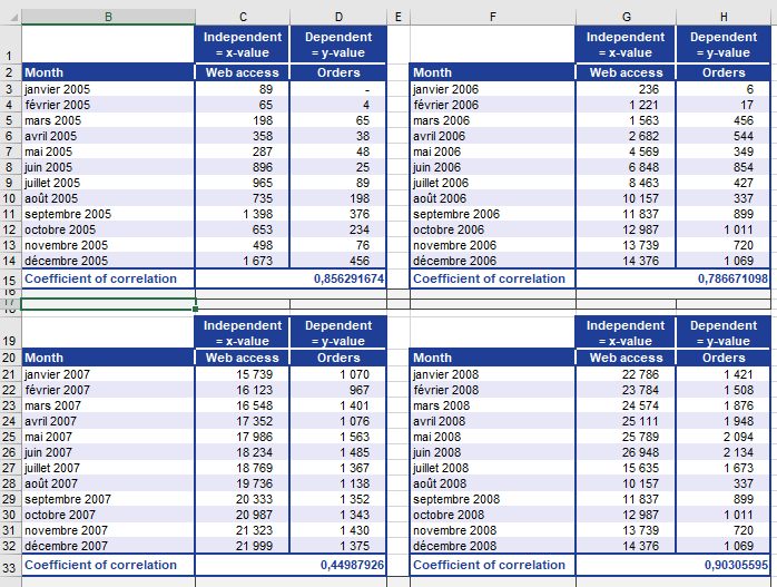
Example: Website Visits vs. Online Orders

Scenario

A software company (founded in 2005) analyzes website visits and online orders (2019–2022) to determine if marketing efforts (e.g., newsletters) drive sales.

Data

• Yearly correlation coefficients (r) between visits and orders (Figure below).
• Problem: Cannot directly average r values (non-interval scaled).

Solution

1. Transform r to z
   • Use FISHER(r) for each year (Figure below).

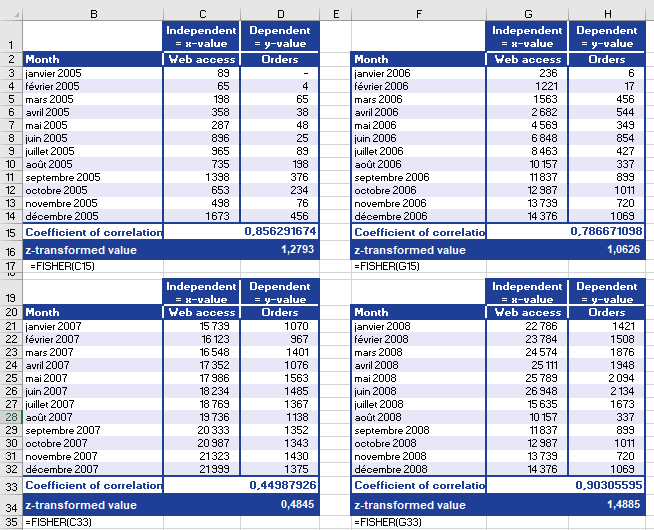
1. Average z-values (Figure below).

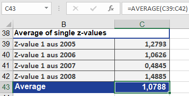
1. Revert to r
   • Apply FISHERINV(z_avg) → Final r = 0.7927 (Figure below).

Interpretation

• r = 0.7927: Strong positive correlation.
  • As website visits ↑, online orders ↑.
• Conclusion: Marketing-driven visits significantly increase orders.

Key Takeaways

• Use FISHER() to:
  • Normalize correlation data for statistical tests.
  • Compute averages of multiple correlations.
• Use FISHERINV() to revert z back to r.
• Limitation: Only valid for -1 < r < 1.

This function returns the test statistic of an F-test, which calculates the one-tailed probability that the variances of two datasets (array1 and array2) are not significantly different.

Syntax

F.TEST(array1; array2)

Arguments

• array1 (required): The first dataset (range or array).
• array2 (required): The second dataset (range or array).

Background

The F.TEST() function determines whether two samples exhibit different variances. For example:

• Compare test scores from public vs. private schools to assess differences in score variability.
• Evaluate whether the variance between two groups is statistically significant.

Key Notes:

1. Purpose: Tests if two sample variances are equal.
2. Output: Returns a significance level (p-value) between 0 and 1 (or 0%–100%).
   • A high p-value (e.g., 0.89) suggests no significant difference in variances.
   • A low p-value (e.g., <0.05) indicates significant differences.
3. Calculation: Directly computes significance from raw data without pre-calculating variances.

Example: Clinical Drug Study

Scenario

• Goal: Test if an increased drug dosage speeds up recovery.
• Groups:
  • Control group: Standard daily dosage.
  • Test group: Higher initial dosage.
• Metric: Treatment duration (days).

Hypotheses

• Null (H₀): No difference in treatment efficacy.
• Alternative (H₁): Higher dosage improves recovery time.

Analysis

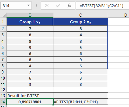
1. F.TEST Result: 0.89 (89%) (see Figure below).

1. • Interpretation: 89% probability that variance differences are due to chance.
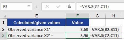
2. Variance Comparison (Figure below):
   • Minor differences between groups.
   • Confirms H₀ (no significant variance difference).

Conclusion

• Retain H₀: No evidence that higher dosage alters recovery time variability.

Key Takeaways

• Use F.TEST() to compare variances of two datasets.
• High p-value (e.g., >0.05): Fail to reject H₀ (variances are similar).
• Low p-value (e.g., ≤0.05): Reject H₀ (significant variance difference).

The F.INV.RT() function returns the inverse of the right-tailed F-distribution. If p = F.DIST.RT(x,…), then F.INV.RT(p,…) = x.

The F-distribution is used in an F-test to compare variances between two data sets. For example, you could analyze income distributions in the United States and Canada to determine whether the two countries exhibit similar income diversity.

Syntax

F.INV.RT(probability; degrees_freedom1; degrees_freedom2)

Arguments

• probability (required): The probability associated with the F-distribution (e.g., significance level α).
• degrees_freedom1 (required): The degrees of freedom in the numerator.
• degrees_freedom2 (required): The degrees of freedom in the denominator.

Background

• The output of an ANOVA (Analysis of Variance) often includes:
  • The F-statistic
  • The F-probability (p-value)
  • The critical F-value at a specified significance level (e.g., 0.05).
• This function helps test whether the means of two or more samples are statistically equal.
• It evaluates if observed differences in group means are significant or due to random variation.

The F.INV.RT() function calculates the critical F-value for a given significance level (α). By comparing this critical value to the calculated F-statistic, you can accept or reject the null hypothesis.

Example

Scenario:
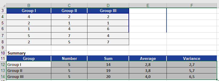
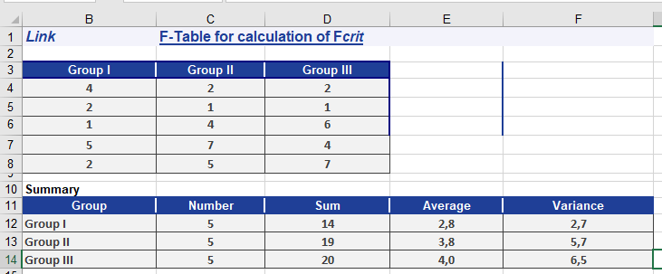
You are an occupational therapist studying how strongly employees identify with their company.

• Sample: 15 employees, each answering 10 questions (with 3 answer options per question).
• Data is summarized (Figure below).

Hypotheses:

• Null hypothesis (H₀): No difference exists between the three employee groups.
• Alternative hypothesis (H₁): A significant difference exists.
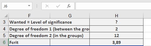
• Significance level (α): 0.05 (5%).

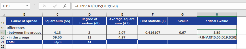
ANOVA Results (Figure below):

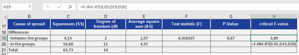
• Between-group variance: Measures differences across groups.
• Within-group variance: Measures random differences among individuals in the same group.

Degrees of Freedom:

• df1 (within groups): (5–1) + (5–1) + (5–1) = 12
• df2 (between groups): 3 groups – 1 = 2

Key Calculations:

1. F-statistic: 0.42 (cell F19).
2. Critical F-value: Calculated via F.INV.RT(0.05, 2, 12).

Conclusion:

• If the F-statistic ≥ Critical F-value, reject H₀.
• Here, 0.42 < Critical Value → H₀ is accepted.
• Interpretation: No significant difference exists between the groups.

Key Notes

• F.INV.RT() computes the threshold F-value for a given α.
• Compare this critical value to your F-statistic to decide on H₀.
• Retain H₀ if F-statistic < Critical Value (no significant difference).

This function returns the values of a distribution function (1 – alpha) of a right-tailed F-distributed random variable. Use this function to determine whether two data sets have different variances.

For example, you can compare the survey results of three equal employee groups to determine whether the variance in results is statistically different.

Syntax

F.DIST.RT(x; degrees_freedom1; degrees_freedom2)

Arguments

• x (required): The value at which to evaluate the function.
• degrees_freedom1 (required): The degrees of freedom in the numerator.
• degrees_freedom2 (required): The degrees of freedom in the denominator.

Background

• The F.DIST.RT() function returns the significance level (probability) based on a given F-value.
• It calculates the probability (significance level) for the critical F-values determined by F.INV.RT().
• The F.INV.RT() function, in contrast, calculates the critical F-value based on a given probability and degrees of freedom.

Example

In a survey, 15 employees answered 10 questions, each with three possible answers (see Figure below).

• Null hypothesis (H₀): No difference exists between the three groups.
• Alternative hypothesis (H₁): A significant difference exists.

A variance analysis returns the results shown in Figure below.

• Using F.INV.RT() with a significance level (α) of 0.05, the critical F-value is calculated as 3.89.
• F.DIST.RT() returns a significance level of 0.05 for this critical value.

The function uses the values from Figure  to compute F.DIST.RT().

The calculation of the significance level for F produces the result shown in Figure below.

• F.DIST.RT() returns a probability of 0.67 (67%) for the test statistic F = 0.4161 (see Figure below).

Since the significance level (α = 0.05) is less than the p-value (0.67), the null hypothesis is not rejected. This means there is no significant difference between the groups.

Key Notes

• F.DIST.RT() calculates the right-tailed probability (significance level) for a given F-statistic.
• If the returned p-value > α, the null hypothesis is retained (no significant difference).
• If p-value ≤ α, the null hypothesis is rejected (significant difference exists).

This function calculates probabilities for an exponentially distributed random variable, modeling the time between independent events. It is commonly used to predict waiting times, such as:

• The time until a call center receives the next call.
• The duration between ATM transactions.

Syntax

EXPON.DIST(x ; lambda ; cumulative)

Arguments

• x (required): The time value for which you want to calculate the probability.
• lambda (required): The rate parameter (average events per time unit).
  • Example: If calls average 3 per minute, lambda = 3.
• cumulative (required):
  • TRUE: Returns the cumulative distribution function (CDF) (probability of an event occurring by time x).
  • FALSE: Returns the probability density function (PDF) (likelihood of an event occurring at exactly time x).

Background

Key Properties

• Memoryless Process: The probability of an event occurring in the next interval is independent of past events.
• Decay/Growth: Models processes where values change by a constant factor over equal intervals (e.g., radioactive decay, call arrivals).
• Inverse: The natural logarithm is the inverse of the exponential function (base *e*, Euler’s number ≈ 2.71828).

Formulas

1. Probability Density Function (PDF):

f(x;λ)=λe−λx(Likelihood at exact time x)

1. Cumulative Distribution Function (CDF):

F(x;λ)=1−e−λx(Probability of event occurring by time x)

Example

Let’s use with the example of the call center. Assume that you operate a call center for a printer manufacturer. The call center is open 24 hours a day, seven days a week. You want to analyze the call pattern and count the incoming calls every hour over one day. This means that the time interval is 60 minutes.

The recorded calls result in the statistics shown in Figure below.

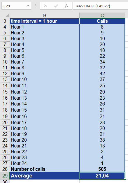
After you have calculated the average of all incoming calls, you can make the following statements:

Every hour, an average of 21 calls come in.

This means that, on average, every three minutes a customer calls.

Now you want to know the probability that a customer will call after two minutes. To find out, you use the EXPON.DIST() function. What information do you have to enter for the arguments?

x = 2, because we want to calculate the probability for a call after 2 minutes.

Lambda = 3, because this is the mean value of events per interval and therefore the passed value.

cumulative = TRUE, because in our example the cumulative distribution should be returned.

Figure below shows the result from the calculation of the probability with the EXPON.DIST() function.

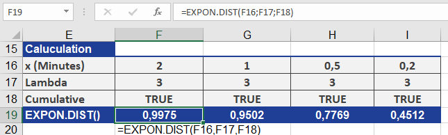
The probability for a call coming in after two minutes is 99 percent.

As you can see in figure above, the probability decreases as the time interval decreases. This means that the probability for a call to come in after

0.2 minutes (12 seconds) is only 45 percent.

Key Notes

• Lambda (λλ): Must match the time unit of x (e.g., if x is in minutes, lambda = events/minute).
• Common Uses:
  • Reliability analysis (e.g., time until failure).
  • Queueing theory (e.g., wait times).
• Visualization: Exponential distributions have a steep decay curve.

This function calculates the sum of squared deviations of data points from their sample mean. It measures the total variability (dispersion) within a dataset.

Syntax

DEVSQ(number1; [number2]; …)

Arguments

• number1 (required): The first numerical value or range.
• number2, … (optional): Additional values or ranges (up to 255 arguments in modern Excel).
• Note: You can use a single array (e.g., A2:A10) instead of comma-separated arguments.

Background

Regression & Correlation

• Correlations between variables are quantified using coefficients (e.g., Pearson’s *r*).
• Regression models predict a dependent variable (*y*) from an independent variable (*x*). A linear model assumes a straight-line relationship (e.g., « as *x* increases, *y* increases/decreases »).
• Model quality is often assessed using R² (the proportion of variance explained by the model).

Forecast Error & Variability

• The mean (average) is the simplest predictor of *y*. Deviations from the mean are called forecast errors.
• Variance (calculated with VAR.S()) averages these squared deviations.
• DEVSQ() sums these squared deviations, providing a raw measure of total variability.

Formula

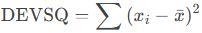
Where:

• xi = Individual data points.
• xˉ = Sample mean (AVERAGE of the data).

Example

Scenario: Analyzing the relationship between website visits (*x*) and online orders (*y*).

• Goal: Calculate the total squared deviations of website visits from their mean to assess data spread.
• Result: DEVSQ () returns 1,109,624,270 (see Figure below), matching the manual sum of squared deviations.

Why Use DEVSQ()?

1. Regression Analysis: Used in calculating SST (Total Sum of Squares) for R².
2. Statistical Tests: Helps evaluate data dispersion (e.g., ANOVA).
3. Quality Control: Monitors variability in processes.

Key Notes

• Difference from VAR.S():
  • VAR.S() divides DEVSQ() by n−1 to compute sample variance.
  • DEVSQ() provides the numerator of variance formulas.
• Units: Output is in squared units of the original data (e.g., « visits² »).

This function calculates the population covariance, which is the average of the products of deviations for each pair of data points. Covariance helps determine the relationship between two datasets. For example, you can analyze whether higher income levels correlate with higher education levels.

Syntax

COVARIANCE.P(array1; array2)

Arguments

• array1 (required): The first range of integer values.
• array2 (required): The second range of integer values.

EXAMPLE

Key Notes

• Population vs. Sample: Unlike COVARIANCE.S (sample covariance), COVARIANCE.P calculates covariance for an entire population.
• Interpretation:
  • Positive result: Indicates a direct relationship (as one variable increases, the other tends to increase).
  • Negative result: Indicates an inverse relationship (as one variable increases, the other tends to decrease).
  • Zero: Suggests no linear relationship.

This function returns the covariance of two sets of values. Covariance helps determine the relationship between two datasets. For example, you can analyze whether an increase in online orders correlates with the number of website visits. To compute covariance, the deviations of all value pairs from their respective means are multiplied, and then the average of these products is taken.

Syntax

COVAR(array1; array2)

Arguments

• array1 (required): The first range of integer values.
• array2 (required): The second range of integer values.

Background

The covariance describes the correlation between two variables, *x* and *y*, in terms of direction (positive or negative). It indicates whether the relationship between the variables is direct or inverse. Covariance can take any real value.

Interpreting Covariance Results

• Positive covariance: Indicates a concordant linear relationship between *x* and *y*. High values of *x* correspond to high values of *y*, and low values of *x* correspond to low values of *y*.
• Negative covariance: Indicates an inverse linear relationship. High values of one variable correspond to low values of the other.
• Zero covariance: Suggests no linear correlation between *x* and *y*.

While covariance reveals the direction of the relationship, it does not measure the strength of the correlation. This is because covariance depends on the scale of the variables. For instance, a covariance of 5.2 meters would be 520 centimeters for the same data in a different unit.

Key Insights from Covariance and Standard Deviations

Given *n* pairs of values (x₁, y₁), (x₂, y₂), …, (xₙ, yₙ), with standard deviations sₓ and sᵧ and covariance sₓᵧ, the maximum possible covariance is the product of the standard deviations (sₓ × sᵧ). This upper limit occurs when the relationship between xᵢ and yᵢ is linear (i.e., y = a + bx).

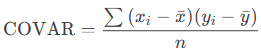
The covariance is calculated as:

COVAR=∑(xi−xˉ)(yi−yˉ)nCOVAR=n∑(xi​−xˉ)(yi​−yˉ​)​

where:

• x̄ and ȳ are the sample means (AVERAGE(array1) and AVERAGE(array2)).
• n is the sample size.

Example

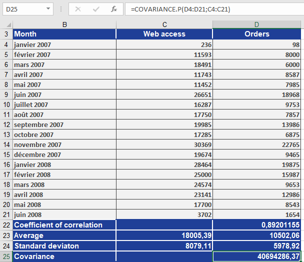
Consider a software company that sells products online and uses newsletters to boost sales. Last year, website orders increased significantly. To understand the reason, you first calculated the correlation coefficient. Now, you want to determine the direction of the relationship between website visits (*x*) and online orders (*y*) by computing the covariance.

The positive covariance confirms a concordant linear relationship—higher website visits correspond to higher orders, and lower visits correspond to fewer orders. This is further supported by a correlation coefficient of 0.89, indicating a strong linear relationship.

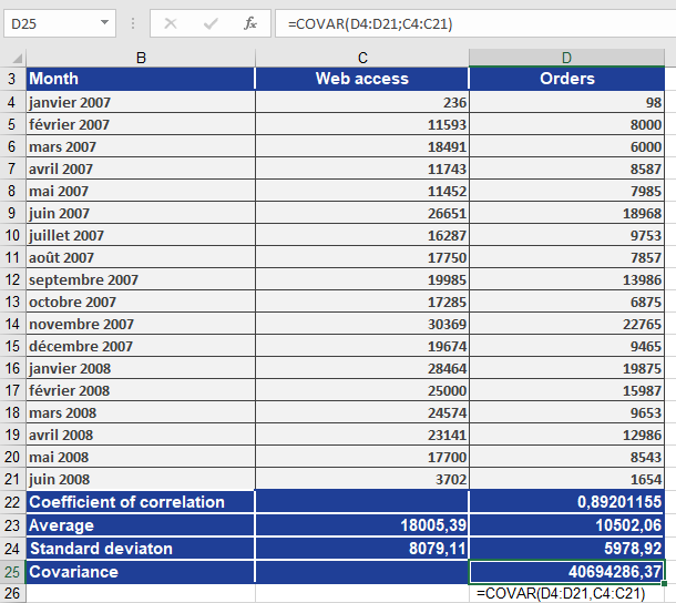
A manual calculation (without COVAR()) using the formula above yields the same result, as illustrated in the accompanying figures.