Votre panier est actuellement vide !
Catégorie : Excel function
How to use the RANK() function in Excel
Returns the rank of a specified number within a dataset, indicating its relative size compared to other values. The rank represents the number’s position if the dataset were sorted.
Syntax:
RANK(number; ref; [order])Arguments
Argument Description number (required) The value to rank. ref (required) The dataset (array or range) containing numbers to compare against. Non-numeric values are ignored. order (optional) Controls ranking direction: - 0 (or omitted): Descending order (highest value = rank 1).
- Non-zero: Ascending order (lowest value = rank 1).
Key Features
- Tied Values:
- Duplicate numbers receive the same rank.
- Subsequent ranks are skipped (e.g., two values tied for rank 3 will omit rank 4).
- Correction for Ties:
To adjust ranks for identical values, use this formula:
text
[COUNT(ref) + 1 – RANK(number, ref, 0) – RANK(number, ref, 1)] / 2
Applies to both ascending and descending rankings.
- Efficiency:
Ideal for large datasets where manual ranking is impractical.
Example: Sales Performance Ranking
Scenario: A software company analyzes monthly sales over two years (24 months).
Steps:
- Data: Column A lists sales figures for each month.
- Ranking:
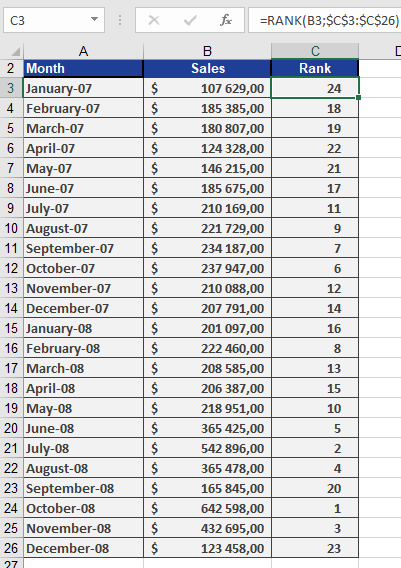
- Use =RANK(A2, $A$2:$A$25, 0) to rank sales in descending order (highest sale = rank 1).
- If sales are unique, ranks span 1–24 without gaps.
Result:
- Column B displays each month’s rank (see Figure below).
- Tied sales would share a rank.
Practical Notes
- Alternatives: Modern Excel versions use RANK.EQ() (identical to RANK()) and RANK.AVG() (assigns average rank to ties).
- Visualization: Combine with conditional formatting to highlight top/bottom performers.
How to use the QUARTILE() function in Excel
Returns the specified quartile of a dataset. Quartiles divide data into four equal groups, useful for analyzing income distributions, sales performance, or survey results (e.g., identifying the top 25% of values).
Syntax:
QUARTILE(array ; quart)Arguments
Argument Description array (required) Range of numeric values to analyze. quart (required) Integer (0–4) specifying which quartile to return. Table 1: Quartile Argument Values
Value Result 0 Minimum value 1 25th percentile (lower quartile) 2 50th percentile (median) 3 75th percentile (upper quartile) 4 Maximum value Key Concepts
- Quartiles split data into 4 equal parts, while quantiles divide it into *n* parts.
- Median (quart=2) divides data into two equal halves.
- For datasets with even observations (e.g., 12 values), the median averages the middle two values.
Pharmaceutical Sales Example
Goal: Analyze pill sales across 5 U.S. regions per 100,000 residents.
Data: 12 monthly sales values per region (sorted in ascending order).
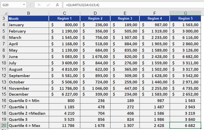
Calculations for Region 1:
- Quartile 0 (Min): $800
- Quartile 2 (Median):
- Position: Between 5th/6th values → (4,200 + 4,220)/2 = $4,210
- Quartile 4 (Max): $11,786
Quartiles 1 & 3 (25th/75th Percentiles):
- Quartile 1 (25%): Between 3rd/4th values → $1,185
- Interpretation: 25% of sales ≤ $1,185.
- Quartile 3 (75%): Between 9th/10th values → $5,525
- Interpretation: 75% of sales ≤ $5,525.
Comparative Insight:
- In Region 5, 75% of sales are ≤ $3,840 (vs. $5,525 in Region 1).
Manual Calculation Notes
- For n=12:
- 25th percentile: 0.25×12 = 3rd/4th values → Weighted toward 4th.
- 75th percentile: 0.75×12 = 9th/10th values → Weighted toward 10th.
Visual Reference: See Figure below for sales data.
How to use the PROB() function in Excel
This function calculates the probability of values falling within a specified range. If no upper limit is provided, it returns the probability of values equaling the lower limit exactly.
Syntax:
PROB(x_range; prob_range; lower_limit; [upper_limit])Arguments:
- x_range(required): The set of possible numerical outcomes.
- prob_range(required): The corresponding probabilities for each value in x_range (must sum to 1).
- lower_limit(required): The minimum value of the target range.
- upper_limit(optional): The maximum value of the target range.
Key Requirements:
- All probabilities must be ≥0 and ≤1.
- The sum of all probabilities must equal 1.
Background:
The PROB() function aggregates probabilities for discrete outcomes. It’s particularly useful when:- Working with known probability distributions
- Analyzing scenarios with defined outcome likelihoods
- Calculating cumulative probabilities for value ranges
Medical Example:
A doctor analyzes patient weight probabilities based on historical data:*Data Setup (Figure below)*:
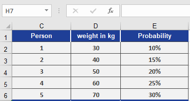
- Weights (x_range): [100, 110, 120, 140, 150] lbs
- Probabilities (prob_range): [0.1, 0.15, 0.25, 0.3, 0.2]
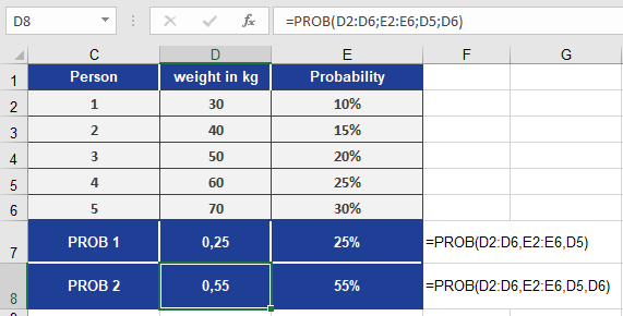
Calculations (Figure below):
- Exact weight probability:
- =PROB(weights, probs, 120)→ 25%
(Probability of weighing exactly 120 lbs)
- =PROB(weights, probs, 120)→ 25%
- Weight range probability:
- =PROB(weights, probs, 120, 140)→ 55%
(Probability of weighing between 120-140 lbs)
- =PROB(weights, probs, 120, 140)→ 55%
Key Notes:
- When upper_limit is omitted, PROB() treats lower_limit as both min and max.
- The function sums probabilities for all x_values within the specified bounds.
How to use the POISSON.DIST() function in Excel
This function calculates probabilities for a Poisson-distributed random variable. The Poisson distribution is commonly used to predict the frequency of rare, independent events over a specific interval (e.g., call center arrivals per hour or tire failures per 100,000 miles).
Syntax:
POISSON.DIST(x ; mean ; cumulative)Arguments:
- x (required): The number of events to evaluate.
- mean (required): The expected average number of events (λ).
- cumulative (required): A logical value determining the calculation type:
- TRUE: Returns the cumulative probability (0 to *x* events).
- FALSE: Returns the exact probability for exactly *x* events.
Background:
Named after Siméon Denis Poisson (1781–1840), this distribution models rare events in large populations where:- Events are independent (e.g., radioactive decay, customer arrivals).
- The average event rate (mean) is known but the actual occurrences are sporadic.
- The probability of an event is proportional to the interval length.
Key Properties:
- Approximates the binomial distribution for low-probability, high-sample scenarios.
- Requires only the mean (λ) as a parameter (unlike the binomial distribution).
- Assumes events are:
- Rare within the interval.
- Random and independent of prior events.
Formulas:
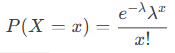
- Exact probability (cumulative = FALSE):
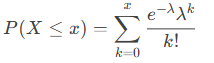
- Cumulative probability (cumulative = TRUE):
Example:
Scenario: A tire dealer observes an average of 4 damage incidents per 100,000 miles.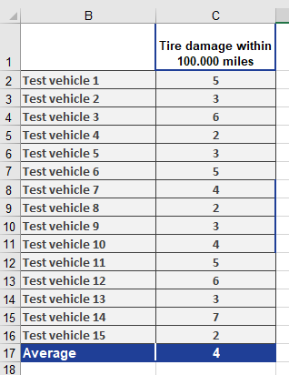
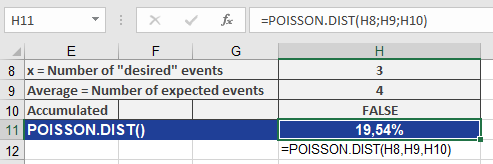
- Question: What is the probability of exactly 3 incidents?
- Inputs:
- x = 3, mean = 4, cumulative = FALSE
- Result: 19.54% (see Figure below).
- Inputs:
- Question: What is the probability of 0 to 3 incidents?
- Inputs:
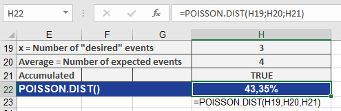
- x = 3, mean = 4, cumulative = TRUE
- Result: 43.35% (see Figure below).
- Inputs:
How to use the PERMUT() function in Excel
This function returns the number of possible permutations when selecting *k* elements from a set of *n* elements. A permutation is an arrangement where the order of elements matters.
Syntax:
PERMUT(number; number_chosen)Arguments:
- number (required): The total number of elements (*n*).
- number_chosen (required): The number of elements to permute (*k*).
Background:
The PERMUT() function belongs to combinatorics, which calculates the number of ordered arrangements. Unlike COMBIN() (where order is irrelevant), PERMUT() treats different sequences as distinct.Key Differences:
- PERMUT(): Order matters (e.g., race rankings).
- Example: Calculating possible podium finishes (1st, 2nd, 3rd) in a 10-runner race.
- COMBIN(): Order irrelevant (e.g., lottery numbers).
- Analogy: Runners would protest if podium places were reordered alphabetically, but lottery numbers remain the same regardless of sequence.
Formula:
The number of permutations is calculated as: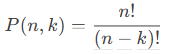
Example:
Scenario: A race with 10 runners (*n = 10*); prizes awarded for 1st, 2nd, and 3rd places (*k = 3*).
Calculation:
=PERMUT(10, 3) returns 720 possible podium arrangements.
This means there are 720 unique ways to assign gold, silver, and bronze medals among the 10 runners.Visual Reference:
See Figure below for the result.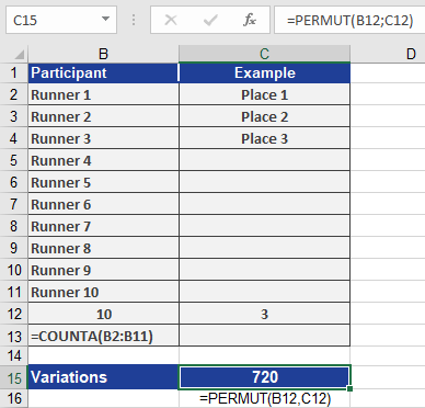
How to use the PERCENTRANK.INC() function in Excel
This function returns the rank of a value (alpha) in a dataset as a percentage, ranging from 0 to 1 (inclusive).
It can be used to evaluate the relative position of a value within a dataset. For example, you can use PERCENTRANK.INC() to assess the standing of an aptitude test score compared to all other test scores.Syntax:
PERCENTRANK.INC(array; x; [significance])Arguments:
- array(required): The array or range of numeric data that defines the relative positions.
- x(required): The value for which you want to determine the rank.
- significance(optional): A value specifying the number of decimal places for the returned percentage. If omitted, INC() defaults to three decimal places (0.xxx).
Background:
PERCENTRANK.EXC() and PERCENTRANK.INC() are the inverse functions of PERCENTILE.EXC() and PERCENTILE.INC(). These functions calculate the relative position of a value *x* within a dataset.
For additional details on quantiles, refer to the PERCENTILE() documentation.Example:
For more details on how to use this function, see the figure below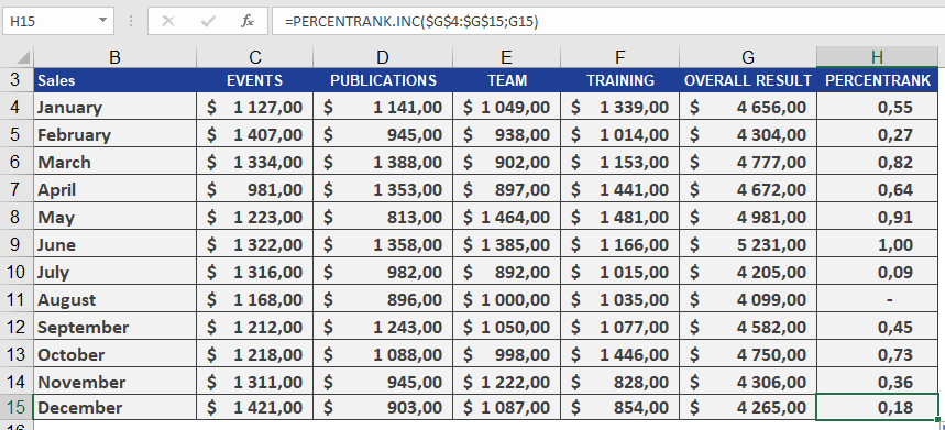
How to use the PERCENTRANK.EXC() function in Excel
This function returns the rank of a value (alpha) in a dataset as a percentage, ranging from 0 to 1 (exclusive).
Syntax:
PERCENTRANK.EXC(array; x; [significance])Arguments:
- array(required): The array or range of numeric data that defines the relative positions.
- x(required): The value for which you want to determine the rank.
- significance(optional): A value specifying the number of decimal places for the returned percentage. If omitted, EXC() defaults to three decimal places (0.xxx).
Background:
PERCENTRANK.EXC() and PERCENTRANK.INC() are the inverse functions of PERCENTILE.EXC() and PERCENTILE.INC(). These functions calculate the relative position of a value *x* within a dataset.
For additional details on quantiles, refer to the PERCENTILE() documentation.Example:
For more details on how to use this function, see the figure below.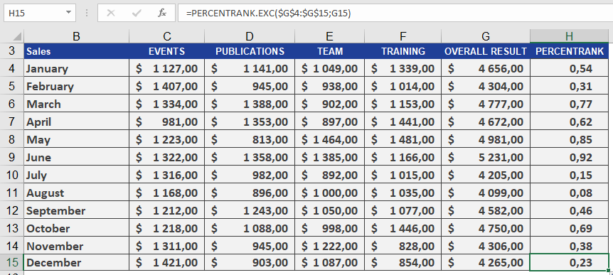
How to use the PERCENTRANK() function in Excel
This function returns the rank of a value (alpha) as a percentage. It can be used to evaluate the relative position of a value within a dataset. For example, you can use PERCENTRANK() to assess the standing of an aptitude test score compared to all other test scores.
Syntax:
PERCENTRANK(array; x; [significance])Arguments:
- array(required): The array or range of numeric data that defines the relative positions.
- x(required): The value for which you want to determine the rank.
- significance(optional): A value specifying the number of decimal places for the returned percentage. If omitted, PERCENTRANK() defaults to three decimal places (0.xxx).
Background:
PERCENTRANK() is the inverse of PERCENTILE(). It calculates the relative position of a value *x* within a dataset. For more details on quantiles, refer to the PERCENTILE() documentation.Example:
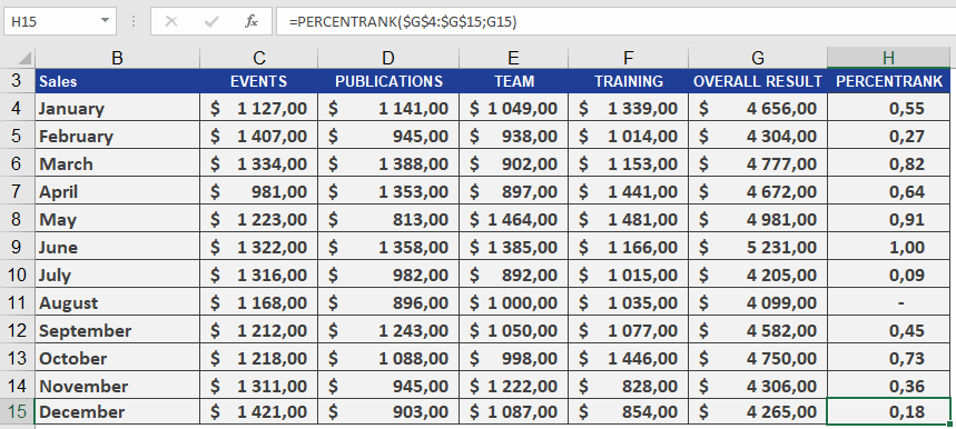
As the manager of the controlling department, you want to analyze the annual sales of all business units. Your goal is to determine the percentile rank of a given month’s sales compared to all monthly sales on a scale from 1 to 100, helping you assess sales variance.Using PERCENTRANK(), you find that January’s sales of $4,656.00 have a quantile rank of 0.55. This means:
- The sales value ranks at 55on a scale of 1 to 100.
- 55%of all monthly sales are less than or equal to $4,656.00, while 45% are greater than or equal to this value (see Figure below).
How to use the PERCENTILE() function in Excel
Returns the alpha quantile (a threshold value) of a dataset, where alpha is a decimal between 0 and 1. This helps identify cutoff points (e.g., « Top 20% of sales »).
Syntax:
PERCENTILE(array; alpha)
Arguments:
- array (required) – The dataset (numeric range) to analyze.
- alpha (required) – The percentile (e.g., 0.8 for 80th percentile).
Background:
- Quantiles split data into ordered segments:
- Median = 0.5 quantile (50th percentile).
- Quartiles = 0.25, 0.5, 0.75 quantiles.
- Deciles = 0.1, 0.2, …, 0.9 quantiles.
- Calculation Rules:
- If n * alpha is not an integer, round up to the next data point.
- If n * alpha is an integer, interpolate between adjacent values.
(Example: For 16 data points, the 0.25 quantile falls between the 4th and 5th values.)
Example:
A software company analyzes annual sales across business units to identify top performers:
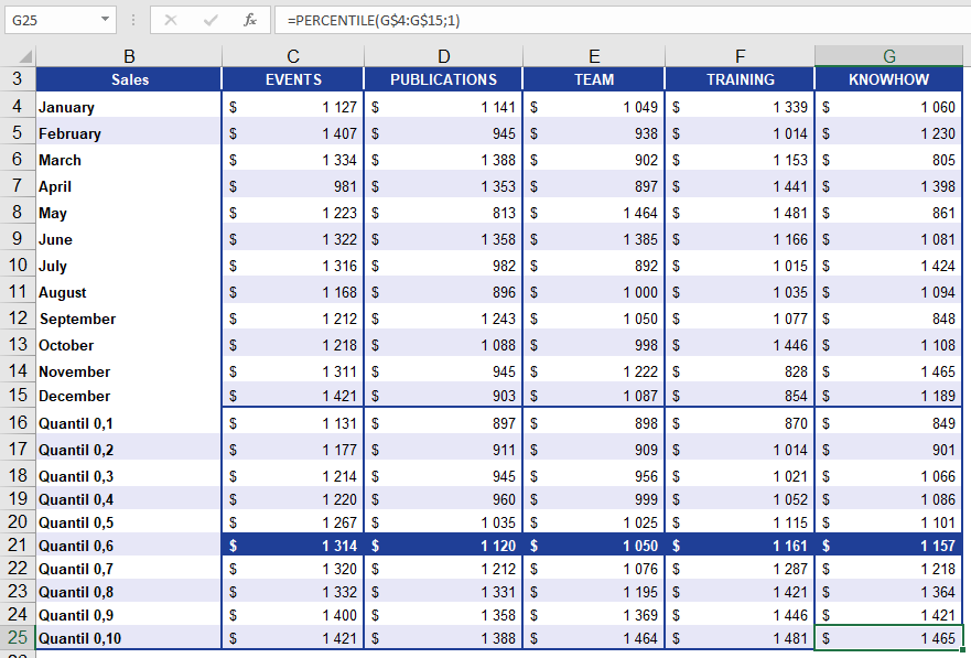
- 60% of sales values are below the returned threshold.
- 40% of sales values are at or above it.
Key Notes:
- Practical Use: Flag high-performing segments (e.g., « Invite customers above the 80th percentile to an event »).
- Limitation: Requires sorted data for manual validation.
How to use the PEARSON() function in Excel
Returns the Pearson correlation coefficient (*r*), a dimensionless value between –1.0 and 1.0 that quantifies the linear relationship between two datasets.
Syntax:
PEARSON(array1; array2)
Arguments:
- array1 (required) – Independent variable (*x*) values.
- array2 (required) – Dependent variable (*y*) values.
Background:
- Interpretation of *r*:
- +1: Perfect positive linear correlation.
- –1: Perfect negative linear correlation.
- 0: No linear correlation.
- Limitations:
- Only measures linear relationships (ignores nonlinear patterns).
- Does not imply causation.
- Formula:
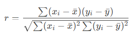
Where xˉ and yˉ are the means of array1 and array2.
Example:
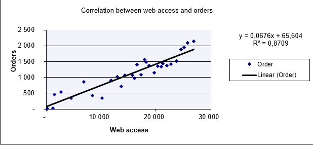
A software company analyzes the relationship between website visits (x) and online orders (y).
- Scatter Plot (Figure below): Visual linear trend suggests correlation.
- Calculation:
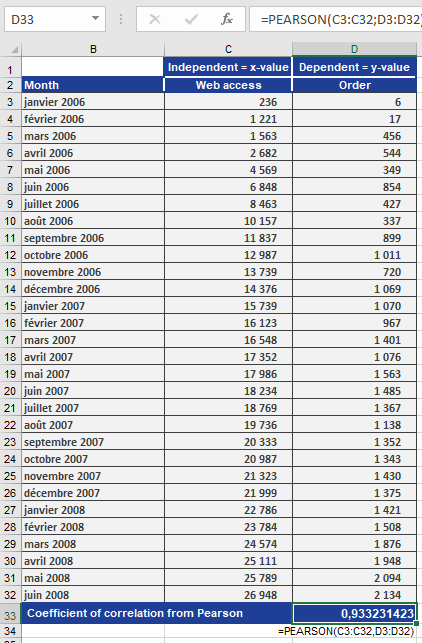
=PEARSON(B2:B100, C2:C100) // Returns r = 0.933
Result (Figure below):
-
- r=0.933r=0.933 → Strong positive correlation.
- Interpretation: Increased website visits closely align with increased orders.
Key Notes:
- High *r* ≠ Causation: Confounding factors (e.g., marketing campaigns) may influence results.
- Always visualize data (e.g., scatter plots) to validate linearity.