Catégorie : Excel function

This function returns the z-value (quantile) of the standard normal distribution (mean = 0, standard deviation = 1) for a given cumulative probability.

Syntax:

NORM.S.INV(probability)

Arguments:

• probability (required) – A cumulative probability (0 < p < 1) associated with the standard normal distribution.

Background:

• The NORM.S.INV() function is the inverse of NORM.S.DIST().
• It calculates the z-value (standardized score) corresponding to a given cumulative probability (area under the curve to the left of *z*).
• The standard normal distribution has:
  • Mean (μ) = 0
  • Standard deviation (σ) = 1

Example:

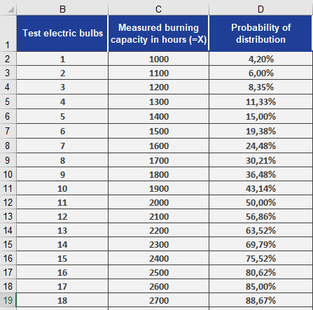
Using the light bulb lifespan data from previous examples (STANDARDIZE() and NORM.S.DIST()):

• You have already calculated probabilities for performance values (see Figure below).

• To find the z-values for these probabilities:

=NORM.S.INV(D2)  // Returns z-value for the probability in cell D2

Results (see Figure below):

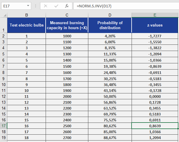
• The function converts probabilities (e.g., 0.042) back to their standard normal distributed z-values (e.g., –1.728).
• Interpretation: A probability of 4.2% corresponds to z = –1.728, meaning 4.2% of bulbs fall below this standardized lifespan.

Key Notes:

1. Inverse Function: Maps probabilities back to z-scores, unlike NORM.S.DIST() (which maps z-scores to probabilities).
2. Standard Normal Only: Assumes μ = 0 and σ = 1 (use NORM.INV() for non-standard distributions).

This function returns the probability (either cumulative or density) for a given z-value in the standard normal distribution (mean = 0, standard deviation = 1). It eliminates the need for traditional statistical tables.

Syntax:

NORM.S.DIST(z ; cumulative)

Arguments:

• z (required) – The quantile (standardized value) for which the probability is calculated.
• cumulative (required) – A logical value determining the output:
  • TRUE: Returns the cumulative distribution function (CDF).
  • FALSE: Returns the probability density function (PDF).

Background:

The standard normal distribution has:

• Mean (μ) = 0
• Standard deviation (σ) = 1

Its density function is given by:

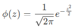
• CDF (cumulative = TRUE): Returns P(Z≤z)(e.g., the area under the curve to the left of *z*).
• PDF (cumulative = FALSE): Returns the height of the curve at *z*.

Example:

Using the light bulb lifespan data from the STANDARDIZE() example:

• Measurements are standardized to z-values (e.g., –1.728 in cell D2).
• To find the probability for each z-value:

=NORM.S.DIST(D2, TRUE)  // Returns cumulative probability

Results (see Figure below):

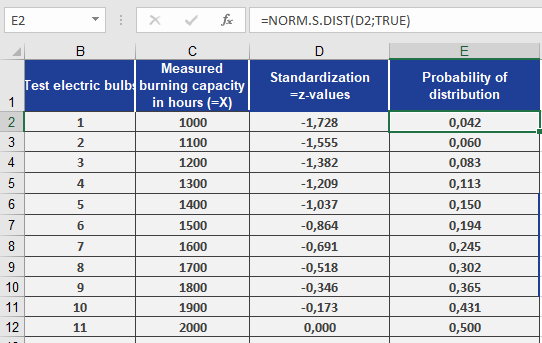
• For z = –1.728, the probability is 4.2% (cell E2).
  Interpretation: Only 4.2% of bulbs have a lifespan ≤ this z-value.

This function returns the quantile (inverse of the cumulative distribution) of a normal distribution for a given probability, mean, and standard deviation.

Syntax:

NORMINV(probability; mean; standard_dev)

Arguments:

• probability (required) – A probability value (0 ≤ *p* ≤ 1) associated with the normal distribution.
• mean (required) – The arithmetic mean (µ) of the distribution.
• standard_dev (required) – The standard deviation (σ) of the distribution.

Background:

A standard normal distribution has:

• Mean (µ) = 0
• Standard deviation (σ) = 1

Any normal distribution can be converted to a standard normal distribution using:

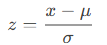
Conversely, a value () in a normal distribution can be derived from a z-score using:

x=μ+z⋅σ

For the standard normal distribution (see Figure below):

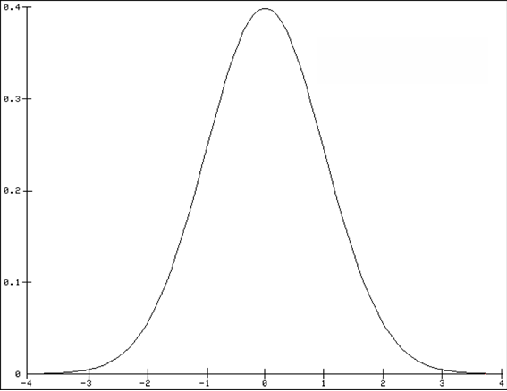
• 68% of values fall within ±1σ of the mean.
• 95.5% of values fall within ±2σ of the mean.
• 99.7% of values fall within ±3σ of the mean.

These same percentages apply to all normal distributions, regardless of µ and σ.

Example:

You are a light bulb manufacturer analyzing lifespan data:

• Mean (µ) = 2,000 hours
• Standard deviation (σ) = 579 hours

You want to find the lifespans for the top 85% and bottom 15% of bulbs.

Using NORMINV():

• 85th percentile: =NORMINV(0.85, 2000, 579) → ~2,600 hours
• 15th percentile: =NORMINV(0.15, 2000, 579) → ~1,400 hours

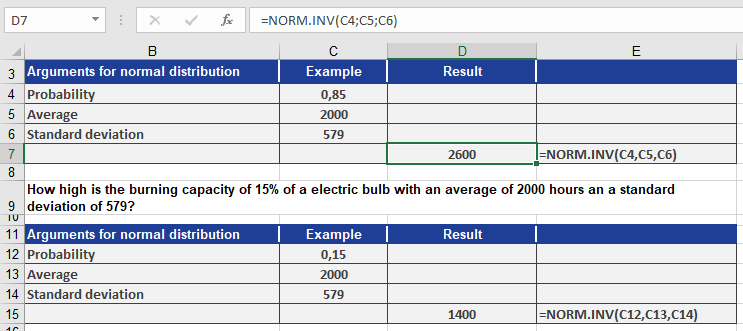
Interpretation (see Figure above):

• 85% of bulbs last up to 2,600 hours.
• 15% of bulbs last up to 1,400 hours.

This function returns the normal distribution for a specified average value and standard deviation. It has broad applications in statistics, including hypothesis testing.

Syntax. NORM.DIST(x, mean, standard_dev, cumulative)

Arguments

• x (required): The distribution value (quantile) for which you want to calculate the probability.
• mean (required): The arithmetic mean of the distribution.
• standard_dev (required): The standard deviation of the distribution.
• cumulative (required): A logical value indicating the type of distribution:
  • If TRUE, the function returns the cumulative distribution function (CDF).
  • If FALSE, the function returns the probability density function (PDF).

Background.
Excel provides numerous statistical functions to calculate distributions and test hypotheses. One such function is NORM.DIST(). In general, distribution functions help answer probability-related questions.

For example, a coin toss has two outcomes: heads or tails.

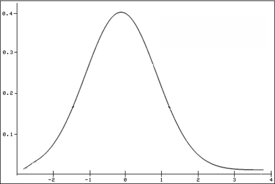
The NORM.DIST() function specifically returns the normal distribution of a given value. The normal distribution is the most important continuous probability distribution, indicating the probability of a random variable x. This distribution is also referred to as the Gaussian function, Gaussian bell, or bell curve, and is shown in Figure beow.

Mathematical Formula (for cumulative = FALSE):

The probability density function (PDF) of the normal distribution is:

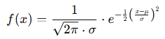
Where:

• x = value in the distribution (quantile)
• μ = mean (average)
• σ = standard deviation
• e = Euler’s number (approx. 2.71828)

If cumulative = TRUE, the formula computes the integral of the above expression from negative infinity up to xxx, yielding the cumulative probability.

Additional Notes on the Normal Distribution:

• It is bell-shaped.
• It is unimodal (has one peak).
• It is symmetrical around the mean.
• It asymptotically approaches the x-axis.
• The maximum occurs at the mean.
• 50% of values lie on either side of the mean.
• Mean, median, and mode are equal.
• Inflection points are located at μ±σ\mu \pm \sigmaμ±σ.

Excel provides both:

• A function ending in DIST to calculate the probability of a value.
• A function ending in INV to calculate the value for a given probability.

Example.
You’re a light bulb manufacturer analyzing bulb lifespans. You’ve determined:

• Mean (μ) = 2,000 hours
• Standard Deviation (σ) = 579 hours

You use NORM.DIST() to evaluate the probability that a bulb lasts:

• Up to 2,600 hours
• Only 1,400 hours

Use:

• cumulative = TRUE → for cumulative probability
• cumulative = FALSE → for exact probability (density)

So for:

• x=2,600x = 2,600x=2,600, NORM.DIST(2600, 2000, 579, TRUE)
• x=1,400x = 1,400x=1,400, NORM.DIST(1400, 2000, 579, TRUE)
• Exact: use the same x values, but set cumulative = FALSE.

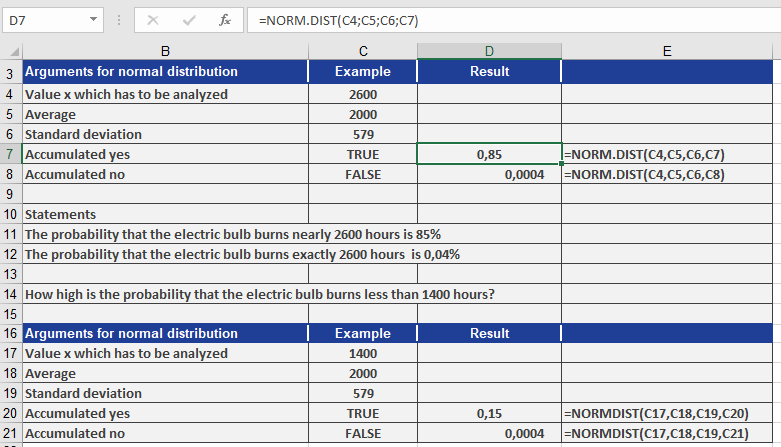
Conclusions from Figure above:

• The probability a light bulb works up to 2,600 hours: 85%
• The probability it works exactly 2,600 hours: 0.04%
• The probability it works only 1,400 hours: 15%
• The probability it works exactly 1,400 hours: 0.04%

With this method, you can:

• Perform hypothesis tests
• Calculate probabilities
• Determine value ranges for various confidence intervals

This function returns the probability of a negatively binomial-distributed random variable. NEGBINOM.DIST() calculates the probability that there will be number_f failures before the number_s-th success occurs, given a constant probability of success probability_s.

Syntax

 NEGBINOM.DIST(number_f; number_s; probability_s)

Arguments

• number_f (required): The number of failures
• number_s (required): The number of successes
• probability_s (required): The probability of a success

Background. This function is similar to the binomial distribution, except that the number of successes is fixed and the number of trials is variable. This is known as a negative binomial distribution. As with the binomial distribution, trials are assumed to be independent.

In a random experiment involving independent repetitions with only two possible outcomes (success or failure), the negative binomial distribution (also known as the Pascal distribution) returns the probability of a fixed number of failures before the x-th success. The formula for the negative binomial distribution is:

where:

• x = number_f
• r = number_s
• p = probability_s

Example. You are on vacation in a foreign city and ask a passerby for directions. Each response can only be « yes » or « no », meaning there is a 50% probability that the answer is « yes ». Therefore, p = 0.5.

After asking several people and receiving no helpful answers, you decide to buy a map. Now, you’re interested in knowing the probability of receiving several “No, I’m sorry” responses before encountering five people who can help. You use the NEGBINOM.DIST() function to calculate this probability, as shown in Figure below.

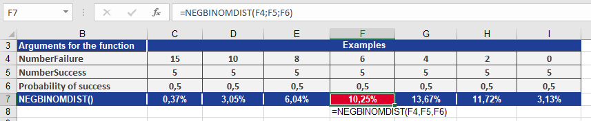
From the result, you can conclude:
With number_f = 6, the probability of asking six people who don’t know the way before you find five people who do is 10.25%.

Returns the most frequently occurring value in a dataset. If multiple values have the same highest frequency, it returns the first one encountered.

Syntax

MODE.SNGL(number1; [number2]; …)

Arguments

• number1 (required): First number, cell reference, or range
• number2,… (optional): Additional values/ranges

Key Features

1. Data Handling:
   • Only considers numeric values
   • Ignores:
     • Empty cells
     • Text entries
     • Logical values
   • Returns #N/A if no duplicates exist
2. Comparison with Other Measures:

Measure	Returns	When to Use
MODE.SNGL	Most common value	Identifying frequent outcomes
MEDIAN	Middle value	Skewed distributions
AVERAGE	Arithmetic mean	Normally distributed data

Example. You are the sales manager of the software company and want to evaluate the number of visits your sales representatives made in different regions numbered 1 through 5: Texas, Virginia, California, Oregon, and Washington. You have already created a table (see figure below).

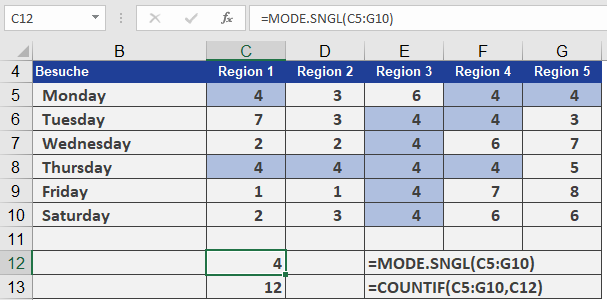
You want to know how many visits were usually necessary before a contract was signed. For this you use the MODE.SNGL() function.

Most of the time, it took four visits to get to the point where the customer signed the contract. If you nest the COUNTIF() and MODE.SNGL() functions, you can also count the number of modes in the range.

The MINA function returns the smallest value in a dataset, evaluating:

• Numbers
• Text representations of numbers
• Logical values (TRUE/FALSE)

Syntax

MINA(value1; [value2]; …)

Arguments

Argument	Requirement	Description
value1	Required	First value, cell reference, or range
value2,…	Optional	Additional values/ranges (1-255 total)

Value Conversion Rules

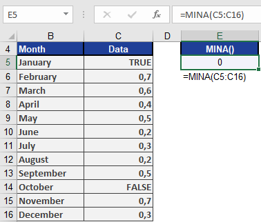
Data Type	Conversion	Example
Numbers	Used as-is	42 → 42
Text numbers	Converted to numeric	« 100 » → 100
Logical TRUE	Treated as 1	TRUE → 1
Logical FALSE	Treated as 0	FALSE → 0
Text strings	Treated as 0	« Text » → 0
Empty cells	Ignored	[blank] → excluded

Example. Using the same example as for MAXA(), the MINA() function returns 0 because the smallest value is the logical value FALSE (see figure below).

Returns the smallest numeric value from a set of arguments.

Syntax

MIN(number1; [number2]; …)

Arguments

• number1 (required): First number, cell reference, or range
• number2,… (optional): Additional values/ranges

Background

• Works identically to MAX() but returns minimum instead of maximum value
• Ignores empty cells, text, and logical values
• Returns 0 if no numeric values are found
• Detailed behavior explained in MAX() function documentation

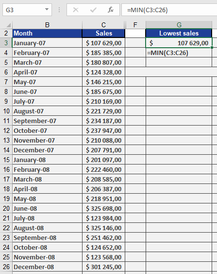
Example. The software company wants to find the smallest number of sales in a given period in a sales table. MIN() returns $107,629 for January from the unsorted data set (see figure below).

Returns the middle value of a numeric dataset when sorted in ascending order. Exactly half of the data points will be greater than the median, and half will be less than the median.

Syntax

MEDIAN(number1; [number2]; …)

Arguments

• number1 (required): First number, cell reference, or range
• number2,… (optional): Additional values or ranges

Calculation Method

1. For odd-numbered datasets:
   • Returns the exact middle value
   • Example: For 5 values → Returns the 3rd sorted value
2. For even-numbered datasets:
   • Returns the average of the two middle values
   • Example: For 6 values → Averages the 3rd and 4th sorted values

Key Properties

• Outlier resistance: Not affected by extreme values
• Data requirements: Works with ordinal or higher measurement scales
• Stability: Insensitive to changes in extreme values
• Missing data: Automatically ignores blank cells and text

Example. Suppose you are the manager of the software company’s marketing department and you want to evaluate the website for the past year. The evaluation includes all clicks in all website areas. Now you want to calculate the median to get the mean value in this data set for the website visits in the past twelve months.

This example calculates the median from the two mean values in the data sets, because the number of elements is even (see figure below).

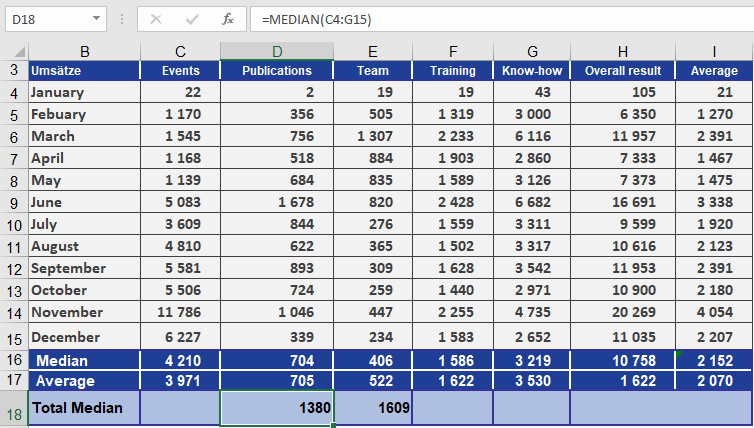
If you sort the events, you can see that the means are July (3,609) and August (4,810). These two values are added by the MEDIAN() function and divided by 2. The result is a median of 4,210. If the example included a  13th month, the median would be the seventh value in the sorted data set

Returns the largest value from a set of arguments, evaluating both numerical and non-numerical data types (including logical values and text representations of numbers).

Syntax

MAXA(value1; [value2]; …)

Arguments

• value1 (required): First value, cell reference, or range to evaluate
• value2,… (optional): Additional values or ranges

Key Features

1. Data Type Handling:
   • Numbers: Evaluated normally
   • Logical values:
     • TRUE = 1
     • FALSE = 0
   • Text representations of numbers: Converted to numerical values
   • Text strings: Ignored (treated as 0)
   • Empty cells: Ignored
2. Comparison with MAX():
   • Unlike MAX() which ignores non-numeric values, MAXA() attempts to convert and evaluate all supported data types
   • Both return 0 if no valid values are found
3. Error Handling:
   • Returns errors if arguments contain unprocessable error values

Example

Scenario:
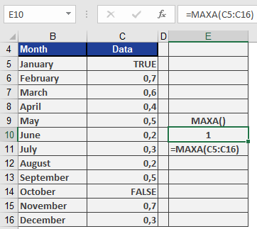
A dataset contains mixed values (numbers, logical values, and text):

Data	Values
A1	0.5
A2	TRUE
A3	« 0.8 »
A4	FALSE
A5	« Text »

Formula:

=MAXA(A1:A5)

Evaluation:

1. Converts values:
   • 0.5 → 0.5
   • TRUE → 1
   • « 0.8 » → 0.8
   • FALSE → 0
   • « Text » → ignored (treated as 0)
2. Compares converted values: (0.5, 1, 0.8, 0)
3. Returns: 1 (from TRUE)

Practical Applications

• Analyzing datasets with mixed data types
• Processing survey data containing logical (Yes/No) responses
• Evaluating conditional results where TRUE/FALSE represent meaningful values

Complementary Functions

• MINA(): Returns smallest value with same conversion rules
• MAX(): Numeric-only maximum function
• COUNT(): Counts numeric values only

Note: For accurate results, ensure text representations of numbers use consistent decimal formats (e.g., « 0.8 » not « 0,8 »).