Votre panier est actuellement vide !
Étiquette : mathematical-and-trigonometry-function
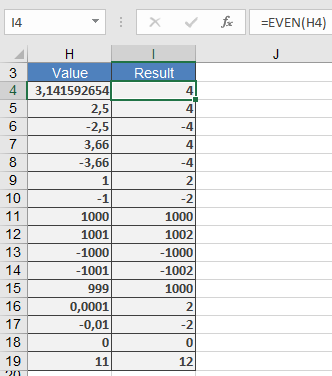
How to use the EVEN() function in Excel
This function rounds a specified number up to the nearest even integer.
Syntax
EVEN(number)Argument
- number (required) – The numeric value to be rounded
- Must be a numeric expression
- Returns #VALUE! error for non-numeric inputs
Background
The EVEN() function performs rounding differently than standard rounding functions:- Always rounds away from zero to the next even integer
- Maintains the sign of the original number
- Returns the input value unchanged if it is already an even integer
- Follows mathematical definition of even numbers (integers divisible by 2)
Key Characteristics:
- Rounding direction:
- Positive numbers: rounds up to next even integer
- Negative numbers: rounds down to next even integer (more negative)
- Special cases:
- Zero (0) is considered even and returns 0
- Exact even integers return themselves
Examples:
Applications:
- Financial calculations requiring even denominations
- Inventory management for paired items
- Team/group formation requiring even numbers
- Data processing with even-number constraints
Error Conditions:
- #VALUE! – Non-numeric input
- #NUM! – Extremely large numbers (Excel limitation)
Related Functions:
- ODD(): Rounds to nearest odd integer
- CEILING(): Rounds to specified multiple
- FLOOR(): Rounds down to specified multiple
- number (required) – The numeric value to be rounded
How to use the DEGREES() function in Excel
Its converts an angle from radians to degrees.
Syntax
DEGREES(angle)Argument
- angle (required) – The angle in radians to be converted
Background
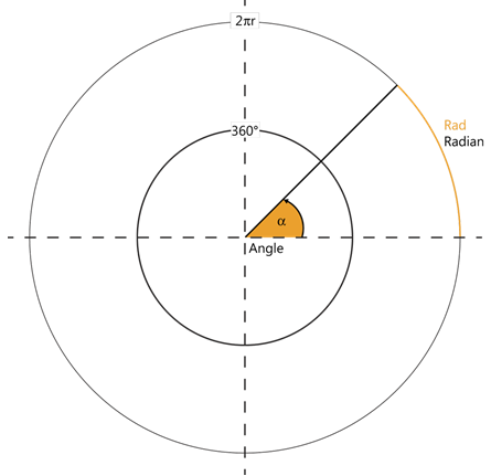
Angular measurements use two primary units:- Degrees (°):
- Full circle = 360°
- 1° = 60 arcminutes (‘)
- 1′ = 60 arcseconds (« )
- Radians:
- Full circle = 2π radians
- π radians = 180°
- 1 radian ≈ 57.2958°
Key Features:
- Essential for interpreting results from Excel’s trigonometric functions (ACOS, ASIN, ATAN, etc.)
- Conversion formula:
degrees=radians×180π
- Inverse function: RADIANS() converts degrees to radians
Examples:
Applications:
- Converting mathematical/engineering calculations to more intuitive degree measurements
- Preparing data for visual presentations/graphs
- Geographic coordinate transformations
- CAD/CAM software inputs
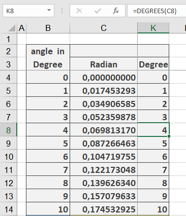
How to use the COSH() function in Excel
This function returns the hyperbolic cosine of a number.
Syntax
COSH(number)Argument
- number (required) – Any real number
Background
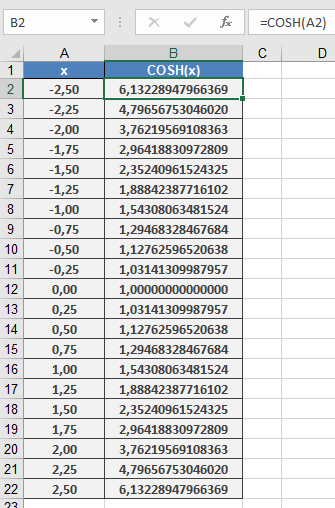
The hyperbolic cosine is part of the family of hyperbolic functions, which – like trigonometric functions – are defined for all real and complex numbers (though Excel only supports real-number arguments). The function is mathematically defined as: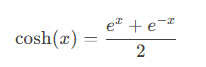
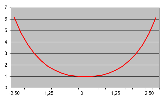
The graph of the hyperbolic cosine (shown in Figure below) displays a characteristic curve.
Example Calculation
Key Applications
- Catenary Curves
The hyperbolic cosine famously describes the shape of a hanging chain or cable suspended between two points (catenary). The catenary equation is:
y = a * COSH(x/a)
where:
-
- a is the vertical distance from the lowest point to the baseline
- x is the horizontal coordinate
- Scientific Uses
- Engineering analysis (suspension bridges, arches)
- Physics (relativity and wave equations)
- Mathematical modeling
Technical Notes
- Output is always ≥ 1
- Symmetric function: COSH(-x) = COSH(x)
- Grows exponentially as |x| increases
- Fundamental relationship: COSH²x – SINH²x = 1
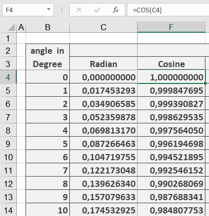
How to use the COS() function in Excel
This function returns the cosine of the specified angle.
Syntax
COS(number)Argument
- number (required) – The angle in radians for which you want to calculate the cosine
Background
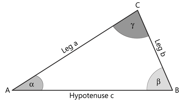
The cosine of an angle in a right triangle represents the ratio of the length of the adjacent side to the hypotenuse (see Figure below):cos(α) = adjacent side / hypotenuse
Key Properties:
- For a unit circle (radius = 1), as angle α increases from 0° to 90°:
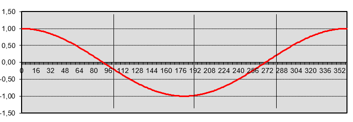
- cos(α) decreases from 1 to 0 (see Figure below)
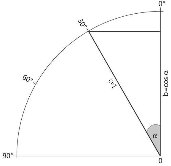
- The cosine function produces a wave-like curve when plotted on a coordinate system (see Figure below)
- The function expects the input angle in radians
- To convert degrees to radians, use the RADIANS() function
Example Application
Additional Notes:
- The cosine function is periodic with a period of 2π radians (360°)
- cos(0) = 1
- cos(π/2) = 0 (90°)
- cos(π) = -1 (180°)
- cos(3π/2) = 0 (270°)
- cos(2π) = 1 (360°)
Common Applications:
- Engineering calculations
- Physics problems involving waves and oscillations
- Computer graphics and game development
- Navigation systems
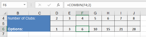
How to use the COMBIN() function in Excel
This function calculates the number of possible combinations (unordered groups) that can be formed from a given set of items.
Syntax
COMBIN(number; number_chosen)Arguments
- number (required) – Total items in the set (must be ≥ 0)
- number_chosen (required) – Items to select in each combination (must be ≥ 0 and ≤ number)
Key Features:
- Returns the binomial coefficient « n choose k »
- Mathematically represented as:
n! / (k!(n-k)!)
- Truncates decimal inputs to integers
- Combination order doesn’t matter (AB = BA)
Error Conditions:
- #VALUE! – Non-numeric arguments
- #NUM! – If:
- Either argument is negative
- number < number_chosen
- Arguments exceed computation limits
Examples:
=COMBIN(4;2) → Returns 6 possible matches
Comparison with PERMUT():
Function Order Matters Formula Example (4,2) COMBIN No n!/(k!(n-k)!) 6 PERMUT Yes n!/(n-k)! 12 Applications:
- Probability calculations
- Tournament scheduling
- Statistical analysis
- Combinatorial mathematics
- Quality control sampling
Note: For large numbers (n > 170), consider alternative methods due to Excel’s factorial computation limits.
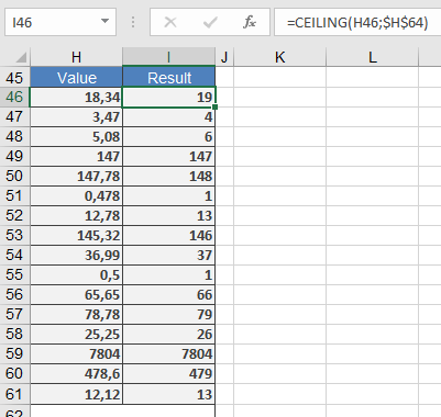
How to use the CEILING() function in Excel
This function rounds a number up to the nearest multiple of the specified significance value.
Syntax
CEILING(number; significance)Arguments
- number (required) – The numeric value you want to round
- significance (required) – The multiple to which you want to round
Key Features:
- Always rounds numbers away from zero
- Handles both positive and negative numbers:
- Positive numbers round up (e.g., 3.2 → 4)
- Negative numbers round down (e.g., -3.2 → -4)
- Returns original value if already an exact multiple
- Returns errors for:
- Non-numeric inputs (#VALUE!)
- Mixed signs between arguments (#NUM!)
Example:
Comparison with Similar Functions:
Function Direction Multiple-Based Handles Negatives CEILING Up (from zero) Yes Yes FLOOR Down (toward zero) Yes Yes MROUND Nearest Yes Yes ROUNDUP Up No Yes How to use the ATANH() function in Excel
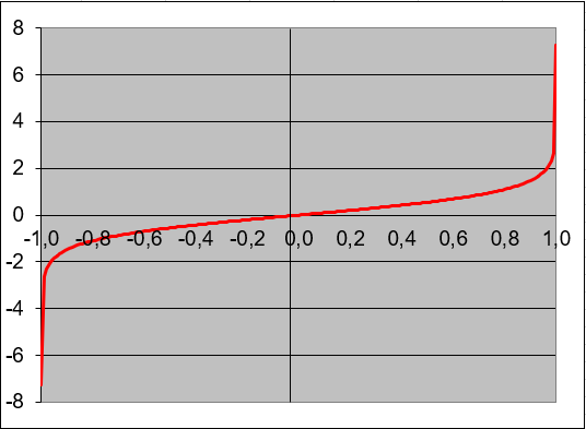
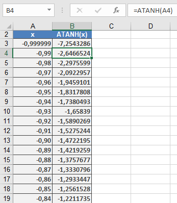
This function returns the inverse hyperbolic tangent of a number. The number must be between -1 and 1 (non-inclusive).
Syntax
ATANH(number)Argument
- number(required) – Any real number strictly between -1 and 1 (-1 < number < 1)
Background
The ATANH() function is the inverse of the hyperbolic tangent (TANH) function. The mathematical formula is:ATANH(x) = 0.5 * ln((1 + x)/(1 – x))
Key Properties:
- Domain: -1 < x < 1
- Range: All real numbers (-∞ to +∞)
- Special Values:
- ATANH(0) = 0
- Approaches ±∞ as x approaches ±1
Examples:
Applications:
- Statistics (Fisher transformation)
- Physics (relativity calculations)
- Engineering (signal processing)
- Financial mathematics
How to use the ATAN2() function in Excel
Its returns the arctangent angle (in radians) between the x-axis and a line from the origin (0,0) to the specified (x,y) coordinates. Unlike ATAN(), this function determines the correct quadrant for the angle.
Syntax
ATAN2(x_num ; y_num)Arguments
Argument Required Description x_num Yes The x-coordinate of the point y_num Yes The y-coordinate of the point Key Features:
- Output Range: -π to π radians (-180° to 180°)
- Conversion to Degrees:
DEGREES(ATAN2(x_num ;y_num))
- Special Cases:
- Returns #DIV/0! if both arguments are 0
- Handles x=0 cases (unlike ATAN(y/x))
Behavior by Quadrant:
Quadrant x_num y_num Result Range I + + 0 to π/2 (0° to 90°) II – + π/2 to π (90° to 180°) III – – -π to -π/2 (-180° to -90°) IV + – -π/2 to 0 (-90° to 0°) 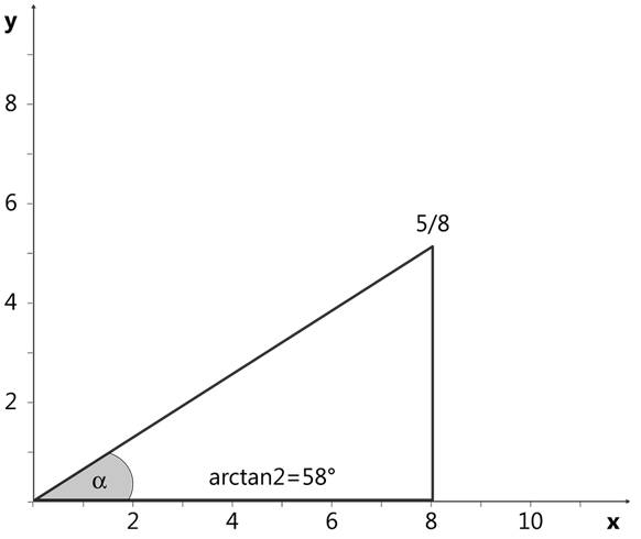
Example:

Comparison with ATAN():
Feature ATAN2() ATAN() Inputs Separate x,y coordinates Single ratio (y/x) Range -π to π (-180° to 180°) -π/2 to π/2 (-90° to 90°) Handles x=0 Yes No Quadrant Awareness Yes No Note: For accurate angle calculations in all four quadrants, ATAN2() is preferred over ATAN() as it automatically adjusts for the correct quadrant based on the signs of both coordinates.
How to use the ASINH() function in Excel
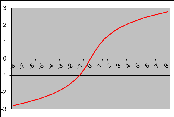
This function returns the inverse hyperbolic sine of a number .
Syntax
ASINH(number)Argument
- number(required) – Any real number
Background
The inverse hyperbolic sine is the inverse function of the hyperbolic sine. The mathematical formula for the inverse hyperbolic sine (sinh⁻¹) is:ASINH(x) = ln(x + √(x² + 1))
Key Properties:
- Defined for all real numbers (-∞ to +∞)
- Output range is unrestricted (-∞ to +∞)
- The function is odd: ASINH(-x) = -ASINH(x)
- Returns values in radians
Examples:
- =ASINH(0)returns 0
- =ASINH(1)returns 0.88137359
- =ASINH(-1)returns -0.88137359

Applications:
- Physics (relativity and wave equations)
- Engineering (signal processing)
- Statistics (transformations of data)
- Geometry (hyperbolic space calculations)
How to use the AGGREGATE() function in Excel
This function returns an aggregate calculation from a list or database.
Syntax. This function has two forms:
AGGREGATE(function_num; options; ref1; [ref2]; …) (reference form)
AGGREGATE(function_num; options; array; [k]) (array form)Arguments
- function_num (required)
A number between 1 and 19 that specifies the aggregation function (see Table 1).
Table 1. Function Numbers and Corresponding Functions
function_num Function 1 AVERAGE() 2 COUNT() 3 COUNTA() 4 MAX() 5 MIN() 6 PRODUCT() 7 STDEV.S() 8 STDEV.P() 9 SUM() 10 VAR.S() 11 VAR.P() 12 MEDIAN() 13 MODE.SNGL() 14 LARGE() 15 SMALL() 16 PERCENTILE.INC() 17 QUARTILE.INC() 18 PERCENTILE.EXC() 19 QUARTILE.EXC() - options (required)
A numerical value that determines which values to ignore (see Table 2).
Table 2. Option Values and Behaviors
option Behavior 0 Ignores nested SUBTOTAL()/AGGREGATE() 1 Ignores hidden rows + nested functions 2 Ignores errors + nested functions 3 Ignores hidden rows, errors, nested functions 4 Ignores nothing 5 Ignores hidden rows only 6 Ignores errors only 7 Ignores hidden rows and errors - ref1 (required for reference form)
The first numeric argument or range for aggregation. - ref2/k (optional)
- Reference form: Additional arguments (up to 253).
- Array form: Required for:
- LARGE(array, k)
- SMALL(array, k)
- PERCENTILE.INC(array, k)
- QUARTILE.INC(array, quart)
- PERCENTILE.EXC(array, k)
- QUARTILE.EXC(array, quart)
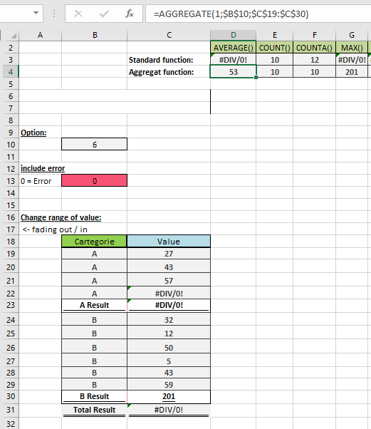
Background. The AGGREGATE() function is a powerful tool introduced in Excel to overcome limitations of other functions. Unlike standard functions that return errors for invalid references, AGGREGATE() provides flexible control over hidden cells and error handling without complex IFERROR() workarounds. It can calculate ranges containing subtotals while excluding them from results (see Figure below).
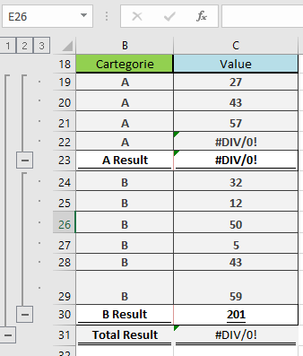
Example. the figure below show an example on aggregate function in excel
- function_num (required)