Étiquette : statistical

The MEDIAN function calculates the middle value of a given set of numbers. For example, the function returns 3 in =MEDIAN(1;2;3;4;5).

The MEDIAN function contains the following arguments:

=MEDIAN(number1; [number2]; …) 

Number1 (Required Argument): The range of one or more cells containing values for median calculation.
Number2 (Optional Argument): Additional numbers to include (up to 255 arguments).

USING THE MEDIAN FUNCTION
Using the table below, let’s calculate the median of numeric data: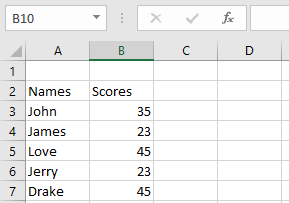

1. Select an empty cell and enter:

=MEDIAN(B3:B7) 

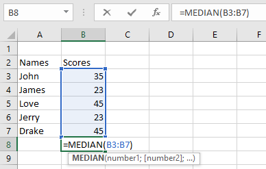
1. Press Enter – the result will be 35 (as shown below).

NOTE: Important MEDIAN function behaviors:

• Returns errors if arguments contain uninterpretable text/errors
• Accepts numbers, named ranges, arrays, or number-containing references
• Ignores empty cells, logical values, and text entries
• For even-numbered sets: returns average of two middle values

The MAX function returns the maximum or largest number in a given set of values or arguments. The MAX function ignores text and logical values in its calculations.

The MAX function uses the following argument:

=MAX(number1; [number2]; …)

Number1 (Required Argument): This is the range of cells from which the highest number will be returned.
Number2 (Optional Argument): Here, up to 255 additional numbers can be included.

USING THE MAX FUNCTION
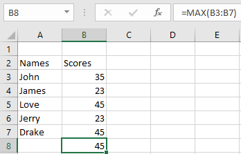
With the table given below, find the maximum number using the MAX function.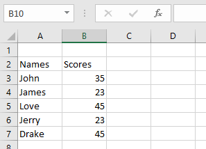

To find the maximum number using the MAX function, follow the steps below:

1. Select an empty cell and type in the function name and its arguments:

=MAX(B3:B7) 

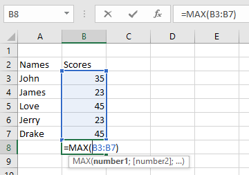
1. Click Enter and the result will be 45 as shown in the table below.

NOTE: Keep these in mind when using the MAX function:

• A #VALUE! error occurs when non-numeric values are provided
• The MAX function returns 0 for arguments without numbers
• To include logical values and text representations of numbers, use the MAXA function
• Arguments can be numbers, names, arrays, or references containing numbers
• Empty cells, logical values, and text are ignored
• Error values or uninterpretable text in arguments will cause errors

The MIN function returns the smallest numeric value from a given set of values. The function ignores text entries and logical values (TRUE/FALSE) in its calculations.

The MIN function uses the following syntax:

=MIN(number1; [number2]; …) 

Number1 (Required Argument): The first number, cell reference, or range containing numeric values to evaluate.
Number2,… (Optional Argument): Additional numbers or ranges to include (up to 255 total arguments).

USING THE MIN FUNCTION
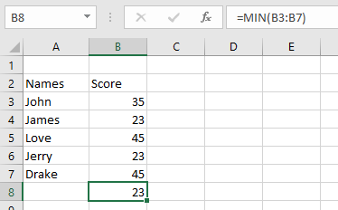
Using the table below, we’ll find the smallest number with the MIN function.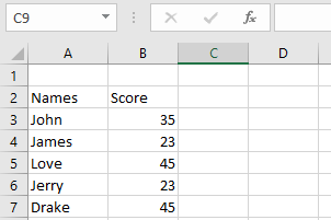

To determine the minimum value:

1. Select an empty cell and enter:

=MIN(B3:B7)   

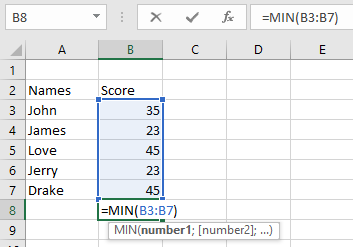
1. Press Enter to display the result: 23 (as shown below).

NOTE: Important MIN function behaviors:

• Returns #VALUE! error if non-numeric data is provided
• To evaluate logical values and text-formatted numbers, use MINA instead
• Accepts numbers, named ranges, arrays, or number-containing references
• Automatically ignores:
  • Empty cells
  • Text entries
  • Logical values
• Returns 0 for arguments without valid numbers
• Returns errors when arguments contain:
  • Uninterpretable text
  • Error values

The AVERAGEIFS function calculates the average (arithmetic mean) of cells that meet multiple specified criteria. This function supports logical operators (<, >, <>) and wildcards (*, ?) in its criteria and was introduced in Excel 2007.

The AVERAGEIFS function uses the following syntax:

=AVERAGEIFS(average_range; criteria_range1; criteria1; [criteria_range2; criteria2]; …) 

Average_range (Required): The range of cells to average (containing numbers, names, arrays, or numeric references).
Criteria_range1 (Required): The first range to evaluate against criteria1.
Criteria1 (Required): The condition for criteria_range1 (number, expression, cell reference, or text).
Criteria_range2, criteria2,… (Optional): Additional ranges (up to 127) and their corresponding criteria.

USING THE AVERAGEIFS FUNCTION
Let’s calculate the average salary of full-time male employees from the table below.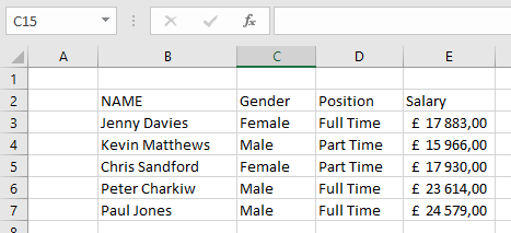

To find this average:

1. Select an empty cell and enter:

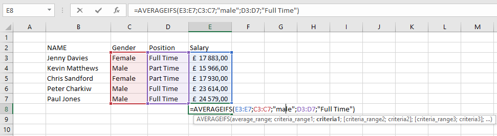
=AVERAGEIFS(E3:E7; C3:C7; « Male »; D3:D7; « Full Time »)

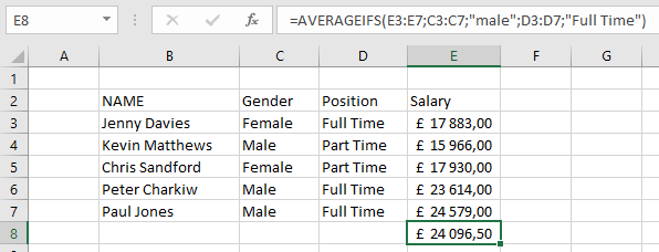
1. Press Enter to display the result: £24 096,50 (as shown below).

NOTE: Key points about AVERAGEIFS:

• Empty criteria ranges are treated as zero
• All criteria ranges must match average_range in size
• Numbers/dates with logical operators must be quoted (e.g., « >4/23/2018 »)
• TRUE/FALSE values evaluate as 1/0 respectively
• #DIV/0! error occurs when:
  • average_range is empty or contains text
  • values can’t be interpreted numerically
  • no cells meet all criteria
• Supports wildcards (*, ?) in criteria

The AVERAGEIF function calculates the average of cells that meet specified criteria. This function supports logical operators (<, >, <>, =) and wildcards (*, ?) in its criteria.

The AVERAGEIF function uses the following syntax:

=AVERAGEIF(range; criteria; [average_range]) 

Range (Required Argument): The set of cells to evaluate, which may contain numbers, names, arrays, or number-containing references.
Criteria (Required Argument): The condition determining which cells to average (can be a number, expression, cell reference, or text – e.g., 13, « <14 »).
Average_range (Optional Argument): The actual cells to average. If omitted, the function uses the range argument.

USING THE AVERAGEIF FUNCTION
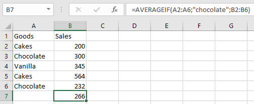
Let’s calculate the average sales of cakes from the table below.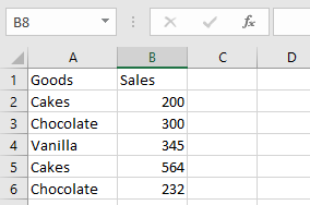

To find the average sales of chocolate cakes:

1. Select an empty cell and enter:

=AVERAGEIF(A2:A6; « chocolate »; B2:B6)

1. Press Enter to display the result: 266 (as shown below).

NOTE: Important AVERAGEIF considerations:

• #DIV/0! error occurs when:
  • No cells meet the criteria
  • The range is empty or contains text
• Criteria referencing empty cells are treated as zero
• Cells with TRUE/FALSE values are ignored
• Supports wildcards (*, ?) in criteria

The AVERAGE function calculates the arithmetic mean of a specified set of values in a worksheet. This function can accept up to 255 arguments, including cell references, ranges, arrays, and constants.

The AVERAGE function uses the following arguments:

=AVERAGE(number1; [number2]; …) 

Number1 (Required Argument): The first number, cell reference, or range for which you want to calculate the average.
Number2 (Optional Argument): Additional numbers, cell references, or ranges to include in the average calculation (up to 255 total arguments).

USING THE AVERAGE FUNCTION
Let’s calculate the average sales of goods in the table below using the AVERAGE function.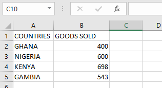

To find the average sales:

1. Select an empty cell and enter:

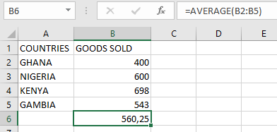
=AVERAGE(B2:B5)

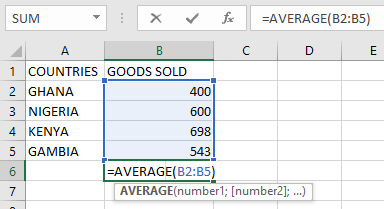
1. Press Enter to display the result: 560,25 (as shown in the table below).

NOTE: Important considerations when using the AVERAGE function:

• Empty cells are automatically excluded from the calculation
• Text and logical values in cell references are ignored
• Cells containing zero (0) are included in the calculation
• All referenced cells must contain numeric values
• To include logical values and text representations of numbers, use the AVERAGEA function
• For conditional average calculations, use the AVERAGEIF or AVERAGEIFS functions

The COUNTBLANK function calculates the number of empty cells within a specified range in a worksheet.

The COUNTBLANK function requires a single argument:

=COUNTBLANK(range) 

Range (Required Argument): This specifies the cell range where blank cells should be counted.

USING THE COUNTBLANK FUNCTION
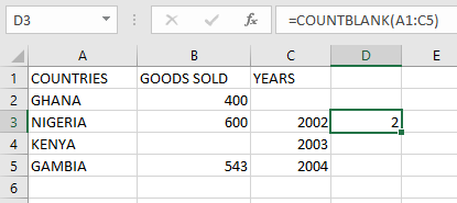
Let’s determine the number of blank cells in the table below using the COUNTBLANK function.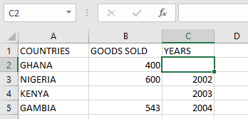

To count blank cells, follow these steps:

1. Select an empty cell and enter:

=COUNTBLANK(A1:C5)

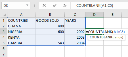
1. Press Enter to display the result: 2 (as shown in the table below).

NOTE: Important notes when using the COUNTBLANK function:

• Excludes cells containing text, numbers, errors, or other non-blank values
• Counts cells with formulas that return empty results as blank
• Does not count cells containing zeros (0) as blank

The COUNTA function is a function that returns the number of non-empty cells within a specified range. This function excludes empty cells from its count. The COUNTA function may also be known as the Excel COUNTIF Not Blank formula.

The COUNTA function uses the following arguments:

=COUNTA(value1; [value2]; …) 

Value1 (Required Argument): This represents the first set of values to be counted.
Value2,… (Optional Argument): These are additional values to include in the count, with a maximum of 255 total arguments permitted.

USING THE COUNTA FUNCTION
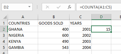
Using the table below, we will determine the number of non-empty cells by applying the COUNTA function.

To calculate the quantity of non-empty cells in your worksheet, follow these steps:

1. Select an empty cell and input:

=COUNTA(A1:C5) 

1. Press Enter to display the result: 15 (as illustrated in the table below).

NOTE: Important considerations when working with the COUNTA function:

• Empty cells are automatically excluded from the count
• For counts excluding logical values, text, or error messages, utilize the COUNT function instead
• To implement conditional counting based on specific criteria, employ either the COUNTIF or COUNTIFS functions

The COUNTIFS function is a function used for counting cells that meet single or multiple conditions or criteria. Just like the COUNT and COUNTIF functions, the COUNTIFS function is used with criteria or conditions relating to numbers, dates, text, logical operators, and wildcards.

The COUNTIFS function has the following arguments:

=COUNTIFS(criteria_range1; criteria1; [criteria_range2; criteria2]…) 

Criteria_range1 (Required Argument): This is the first range to be evaluated with the associated criteria.
Criteria1 (Required Argument): This is the condition to be applied to criteria_range1, which may be an expression, number, cell reference, or text specifying which cells to count. For example, criteria can be expressed as 43, « >23 », D2, etc.
Criteria_range2, criteria2 (Optional Argument): These are additional ranges and their associated criteria. The function allows up to 127 range/criteria pairs. The criteria can be:

• A numerical value (integer, decimal, time, or logical value)
• A text string (e.g., « Monday », « East », « Price ») including wildcards (*, ?)

USING THE COUNTIFS FUNCTION
Using the table below, let’s count the number of shoes that are red.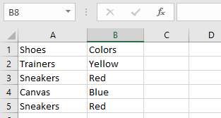

To count red shoes in the list, follow these steps:

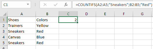
1. Select an empty cell and enter:

=COUNTIFS(A2:A5; « sneakers »; B2:B5; « red »)

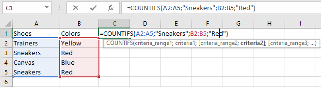
1. Press Enter. The result will be 2, as shown in the table.

NOTE: Remember these points when using COUNTIFS:

• COUNTIFS treats empty cells as 0 when criteria reference an empty cell.
• #VALUE! error occurs if:
  • Criteria ranges have different lengths
  • Text criteria exceed 255 characters
• Wildcards (*, ?) can be used in criteria.
• The function evaluates each cell pair sequentially:
  • If the first cell pair meets criteria, count increases by 1
  • If the second pair meets criteria, count increases again by 1
  • This continues until all cells are evaluated

The COUNTIF function is used to count the number of cells that meet a certain criterion or condition. This can also be used to count cells that contain dates, numbers, and text. This function also supports the use of logical operators and wildcards.

The COUNTIF function has the following arguments:

=COUNTIF(Range; criteria) 

Range (Required Argument): This indicates the range of cells that are to be counted.
Criteria (Required Argument): This is the condition to be met by the cells provided in the worksheet. The criteria can be in the following:

• A numerical value such as integer, decimal, time, or logical value
• A text string such as Monday, East, Price and including wildcards such as asterisks and question mark

USING THE COUNTIF FUNCTION
With the table below, let’s use the COUNTIF function to count how many times James’ name appears on the list.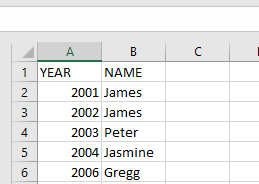

To get the number of times James’ name appears on the list, follow the steps below:

1. Select an empty cell, type in the function name and the arguments to be used:

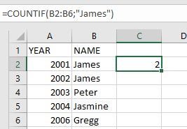
=COUNTIF(B2:B6; « James ») 

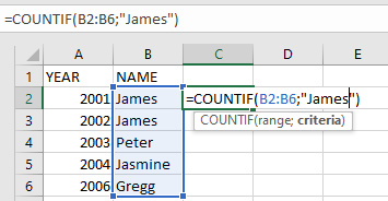
1. Click on Enter and the result will be 2.

NOTE: Take note of the following points when using the COUNTIF function:

• When using the COUNTIF function, make sure the criteria argument is enclosed in quotes (e.g., « James »).
• When the provided criteria argument is a text string that is more than 255 characters in length, #VALUE! error occurs.
• #VALUE! error also occurs when the formula is referring to a cell or range of cells in a closed workbook.